How AI Works - Chapter 4
Neural Networks: Brain-Like AI
We must understand going forward that even though we’ll liken the brain’s neurons to that of connectionist neural networks, they are not the same. Similar, but operate on a totally different level. At a basic level, brain neurons are in an off state until turned on. Artificial neurons are the exact opposite; also containing inputs and outputs but continuously calculating some mathematical function.
A good example is that of a light switch versus a dimming switch. The light switch turns on and off, while the dimming switch varies between different states of being on and producing light. These are the biological and artificial in essence, with some slight overlap that we don’t need to concern ourselves with.
Even the book stresses how important the upcoming figure is to understanding modern AI;
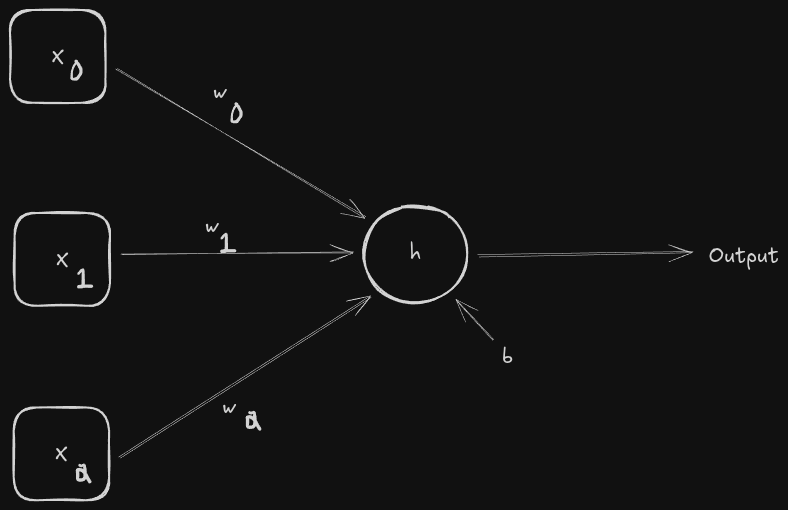
The features are on our left, or the squares containing x. We have a few of them, making up a feature vector. These features flow into the circle h, known as the activation function. Before it gets there however, a weight is introduced that affects each input individually. Not only that, but before the activation function can do its job of producing an output, it has to be affected by b, or bias. The full work of the neuron is like so;
- Multiply each feature by its associated weight
- Add all products from step one with bias to produce a single number
- Give number from step 2 to activation function to produce output
In chapter 2, we learned that the main activation function used in modern networks is ReLU or rectified linear unit. It’s a basic question; is the input less than 0? If so, return 0; otherwise, return the input in whatever way it is. One neuron trained like this is pretty decent for simple inputs, but as in most things in this field, more complex data will call for more a more complex model. Below is a basic example;
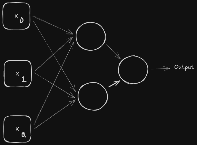
This is a two-node network. Each input connects to each middle layer once, and unlike the last example, these layers connect to one activation node, before producing any output. We could rewrite this as a three-node, four-node, or as many as we want. This new middle layer is called hidden layers. This type of configuration is best for binary classification, or Logistic Regression. Each node within the hidden layer uses ReLU activation functions. There’s a weight for each line from feature to hidden layer, hidden to final, and a bias for each node. Every time we add a node, the weights increase exponentially; most ultra-complex models are made up of thousands of millions of weights.
To give a more direct example as to how this actually works, we’re going to need a dataset. The text provides one, but openly acknowledges that it’s no longer able to access. That’s fine, since our setting is purely theoretical. It’s a grape classification that chooses between two different wines in Italy. All we need to know is 0 or 1; one or the other. We can actually just use the same set-up we have had for our previous examples, since we have three features; alcohol content, malic acid, and total phenols.
Our model is going to take in these three inputs, and see if it can correctly classify the type of wine. Breaking up a training/test split (around 100 training samples and around 25 test samples) the accuracy of our model is about 80% accurate. We’ll go deeper into how the training actually works (I promise) but for now just assume that since we have such little data, it’s a decent score. Lets fill out the diagram we used above to better understand what’s going on;
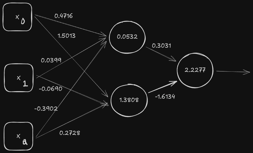
That looks like a lot, and it is! Thankfully, we already broke down most of what’s going on. We know each arrow contains the weighted values we were just talking about. Each circle is not the actual value within it, but the bias value we need to apply to each number before moving on. For example purposes, we’ll use these two points;
- 1. (-0.7359, 0.9795, -0.1333)
- 2. (0.0967, -1.2138, -1.0500)
Each value is complimentary to one of the three features we just discussed (alcohol content, malic acid, and total phenols). You might be considering, how do you have a negative alcohol content? We only have that much because our data went through pre-processing phase, where each feature is given a new value based off of subtracting the average value of how scattered the data is from the overall training dataset (aka standard deviation!). The original value of sample 1’s alcohol is 12.29 percent, but after pre-processing becomes -0.7359.
We can begin walking through this process by taking sample 1’s features, multiplying them to their weights, and sending them to the hidden layer. For example, the top node will be 0.4716 x -0.7359, 0.0399 x 0.9795, and -0.3902 x -0.1333, including the bias value of 0.0532. That’s a lot of numbers, but essentially they’ll give us -0.2028. If you remember how ReLU activation functions work, you’ll know that anything below 0 is sent back as 0, so the top node of the hidden layer will output 0. The bottom node will output 0.1720. Finally, they’ll pass onto the final node gives us 1.9502, which after the sigmoid activation function gives us 0.8755.
If you’ve followed along up till this point, give yourself a well deserved pat on the back. One thing to note going forward is that this output doesn’t give us the label, but a measure of confidence. Neural networks don’t tell us the actual class label for the input, but only their confidence in one label relative to another. So our output is basically going to give us a number from 0 to 1, 0 being no shot and 1 being absolutely. Also, since this is a binary model, it’s giving us the likelihood if it being class 1 (some arbitrary name that does change), meaning our output for sample 1 is that it’s 87% likely to be class 1, instead of the other option. The cut-off point, or where we draw the classification line, is usually 50% for a binary model like this example.
Let’s see if we can figure out the output for the second sample!
Insert work here…
Now that we know the output is 0.4883, we’d probably give that a 49%. Unfortunately for our understanding, that would label it as class 0 instead of class 1. In reality, the sample belongs to class 1, meaning our model was inaccurate. Whether or not this is an acceptable model or not depends upon the context of what it’s used for. In the above example, labeling wine, being wrong 20% of the time is probably bad. But, there are situations where that kind of loss is generally acceptable. If we try to lower our cut-off point, we’re basically switching where our errors are; sometimes there is no way to completely eliminate errors.
What’s nice is that with neural networks, one way we can improve our model is increasing the amount of nodes in our hidden layer. Like the author shows, every time we add another node our percent of accuracy goes up slightly (from 81% to 86%). Our author also explains that when getting these accuracy scores, the test was done 240 times. This is actually something we’ve experienced together in class; every time a training is done for a neural network, the neural networks are randomly initialized. If you think back to our model exercises, you should remember that when we used train_test_split, the split of our data was always different. We had to user the random_state parameter in order to get the same split every time. The same concept applies to neural network models.
One thing I’ve neglected to mention till now is that the weights and biases in the above diagram aren’t set in stone, they are updated in an iterative process. Meaning, as the model gets used, it will start to update the weights and biases to better fit the model and get better output. We don’t want the same values every time we train, and we don’t want them to just be 0. So, how do we actually pick these numbers? For this class, it’s best to think of them as just purely random. We’ll start by picking randomly within a range, and continue to change as our model is trained.
Depending on what initial values were selected, the accuracy score ranges from around 73% to 89%. Neural networks should be trained multiple times in order to catch this range; imagine we got 73% and never tried to get anything better. We’d be stuck with a much worse model. This varying range is also partly due to how small the dataset is, along with there not being many weights and biases; the more weights and biases, along with a larger data set, tend to lean to more consistent training metrics.
Let’s do a quick review of everything we just learned;
- Neural networks are made up of neurons, sometimes called nodes
- Neurons get their output by multiplying the inputs by weights, sum the products, add in a bias value, and pass everything to an activation function
- Neural networks are made up of many neurons (sometimes hundreds of thousands)
- Training a neural network requires assigning a random value to the weights and biases, and are updated iteratively
- Binary neural networks produce binary output (0 or 1) as a measure of confidence
Deeper Dive
We should try and find out where we get these weights and biases; it’s not really enough to say their totally random. Let’s recall that in chapter 2, we learned that neural networks took off thanks to backpropagation and gradient descent. Another concept we should keep in the back of our minds from chapter 3 is optimization, detailed further in SVM’s. The iterative process of updating weights and biases is also an optimization process, but we must always make sure the weights and biases fit general trends in the training data, instead of the actual training data. That probably doesn’t make much sense now, but it will in a second.
Here’s a walk-through of what the training algorithm for a neural network looks like;
- Determine the architecture of your model (# of hidden layers, nodes per layer, activation function, etc.)
- Randomly (but also intelligently!) pick all the weights and biases per node
- Split your training data and send it through for the first time; this will be called the forward pass, and our objective is to calculate the average error
- Backpropagation determines how much each weight and bias effected the average error
- Gradient descent determines what the weights and biases should be updated to (this and the previous step are considered the backward pass)
- Steps 3, 4, and 5 are repeated until the model is deemed sufficient
One concept we haven’t talked about that we just mentioned is this idea of an average error. Keep in mind that in our training data, we know exactly what our output should be. Here’s a basic example; say we know the output of a given input is 1, but our model produces a 0.44. Taking the difference of the expected and actual (1 - 0.44) we get 0.56. That number is the “amount of error”, and it happens to be pretty far away from our anticipated output. Imagine we had gotten 0.96 instead; we’d only have 0.04 error, which is much better.
What we want to do here is find the error for each training sample, and use those to calculate the average error over our entire training set. This average gets used by backpropagation and gradient descent to update our weights & biases. Another term for this average error is called loss, and when I said “deemed sufficient” that usually means the loss is close to 0 as possible.
A weird term that you might here is this term overfitting, which can happen in a neural network quite easily. What this means is that your model learned your training dataset so well that it’s 100% accurate, but has no ability to predict unknown inputs. How do we avoid this happening? First of all, this is usually avoided by having a lot of training data. Another way, if getting more data isn’t possible, is to work on your training algorithm to have it implement weight decay, or penalization to the model for making a weight too large.
One other way is called data augmentation, which sounds like it wouldn’t work. Essentially, you’re creating dummy data based off of your actual training data. A simple example the text gives is taking picture of a dog, and augmenting it by slightly editing the picture; moving the dog up and to the left a bit, removing pixels, etc. Another term for what data augmentation is regularizer, since it helps us regulate our model & avoid overfitting.
Finally, back at the point that’s probably been bugging you this entire time. How do we pick our initial values? Well, I already got into how we just sort of pick a small random number and hope it pans out okay. This is actually how it was done for many years, and was expectedly not so great. Nowadays we have a more structured method of picking these values. There are three different factors that scientists consider before choosing their initial values;
- Form of the activation function (ReLU, sigmoid, etc.)
- Amount of connections from layer below (fan-in)
- Amount of outputs to layer above (fan-out)
There are a couple of formulas that consider these three factors in the weight-deciding process, but we don’t have to get into those right this minute. Bias values are almost always set to 0 and adjusted accordingly. This approach lead to huge leaps in model productivity.
Gradient Descent
We already went through Gradient Descent together, but it doesn’t hurt to freshen up/hear from another persons perspective. I really like the example the text provides, which I’ll condense here. Imagine you are on a hill, and you want to go to a nearby town that is north of your current position. Unfortunately, if you head straight north, you fall of the mountain. If you go north-east, you’ll get to the town eventually but it might take a while due to how slow and flat the path is. Instead, there’s a north-west route, that’s a decent in-between dropping off too fast or too slow. However, since you’re moving down a mountain and off the beaten-path, you probably want to stop every couple of yards or so to make sure you’re still on track. This in a nutshell is how Gradient Descent works.
Gradient Descent will train our model by adjusting the weights and biases of our network. It’s attempting to minimize the error when training on a dataset. The hillside you’re “walking” through is a representation of the error function, and your current position corresponds to the average error. Your objective of the village in the north is the smallest error possible in the network on that given training dataset. It is, as we know, an optimization algorithm. However, this is contradictory to what we actually want out of this model, right? We’re not really looking for the smallest error when making a model, we’re looking to make sure our model can handle unknown inputs.
One concept we know about from our last note on the algorithm is how it will use slope to determine exactly where to go. Gradient Descent will look for the global minimum, or the lowest point on the line where the slope is 0, or no slope. There can often be a few points where the slope is 0, known as local minima. Our algorithm must be able to tell what is and what isn’t the global. It will grab a point on the curve (an x value) and pick a step size dependent on the slope from the point grabbed. When it gets to two dimensions, we have to start considering the maximum gradient, but for the sake of this being an introductory class, we don’t have to go further than a single dimension.
One quick concept that leads into our next algorithm is how it chooses the gradients to move down by. The gradients are what represents the overall effect the weights and biases have towards the total error, meaning as steps are taken and weights & biases are changed, the algorithm keeps track of how much that change to each feature changed the overall error. So how does Gradient Descent choose these values to move down by?
Backpropagation
Put simply, the algorithm called backpropagation comes from differential calculus. That type of math is concerned with how one thing changes as something else changes, like speed. It’s a perfect analogy since it’s almost what backpropagation does; the algorithm outputs to Gradient Descent how make to change in either direction to the weights and biases each step it takes. Now we have everything it takes to respond when someone asks us how neural networks are trained;
Gradient descent is an algorithm that moves in a given direction based on the output of backpropagation, affecting the n weights & biases in order to reduce error for the training set.
Chapter Summary
Neural networks are made up of nodes, and these neural networks end up being responsible for a good amount of machine learning and AI developments. They output a single number, and are made up of many hidden layers depending on the amount of features in a training set. Every time you run one, each model’s weights and biases are randomly selected leading to a different performance each run. Gradient descent and backpropagation are the two algorithms that help make all of this happen.
Next: Chapter 5