Gradient Descent
This one will be a quick one, but it’s really important. We know that given an input dataset, and given a function, we can calculate the output. For example, if we have $x=[1, 2, 3]$, and the function $y=3x-2$, we could reasonably figure out the dataset of $y$; $[1, 4, 7]$. Another term for this function, in the case of Machine Learning, is a prediction function.
Sometimes, we’re only given the input and output data. It would be incredibly helpful if we were able to figure out that prediction function, so we can predict unseen input values with precision. We’re actually going to continue working with the dataset we began working with in single variable linear regression.
To start, we know that in the last lesson we were able to figure out the predicted price given some input value(s). This time, let’s think about it from a graphical standpoint;
Given this graph, how could we draw a line of best fit?
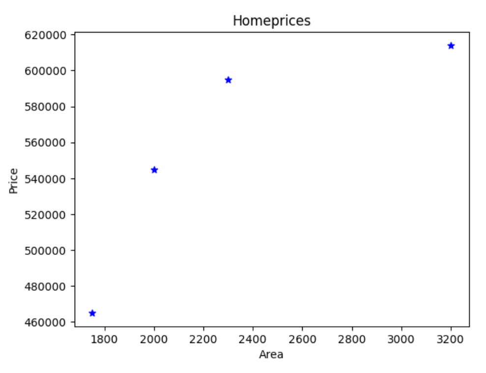
Not only did I choose pretty scattered data points, there are many different ways you could try and attempt to draw your line of best fit. However, your main objective is still the same; minimize the amount of error between the predicted and expected amount.
The above definition actually has a name; it’s called Mean Squared Error. Here’s the formula;
$mse=\frac{1}{n}\sum^{n}{i=1}(y_i-y{predicted})^2$
Looks like a lot, but it’s not that much. $n$ is the amount of data points we have (in our above example, $n=4$ ) and we’re getting the sum of all of the actual values of y versus the expected values of y, squared (we square them to avoid skewed results!). We could also call this formula a cost function. There are different types of cost functions, but MSE is a popular one to begin with. We can rewrite the above equation as;
$mse=\frac{1}{n}\sum^{n}_{i=1}(y_i-(mx_i+b))^2$
Obviously, guessing and checking every combination of $m$ and $b$ is inefficient and will take you forever. This is where our topic of conversation comes into play. Gradient Descent is a machine learning algorithm that calculates the line of best fit for a training data set. Conceptually this is a little weird; if you plot the values of $m$ and $b$ against the MSE (or in this case, cost), you’ll actually get a ball-like graph like in the image reference below.

We start at a point, usually (0,0). We calculate the cost, then reduce the value of $m$ and $b$, and again calculating the cost. We continue to do this until we reach the bottom, or the minima, where the error is minimum. That is our answer, or we’ll use that $m$ and $b$ for our function.
How do we calculate the steps we need to take as we travel down? We don’t want to miss our minima, and if we’re going at a constant rate down, we could eventually miss our minima and never know. A better approach would be to gradually lower the amount decreased as we go on by incrementally smaller steps. How do we know how much to go down by?
Without going too deep into calculus, we are essentially calculating our slope as we go down. How this is done is using derivatives, which you can find a more detailed description on in the resources below. To calculate the next step, you subtract a learning rate value multiplied by the partial derivative of either $m$ or $b$, depending on which one you’re trying to find. Here’s a very oversimplified walk through of how this whole procedure works;
- We start by setting a variable for $m$ and $b$, which by default 0 is a fine value
- Set a value for the amount of iterations. We can pick 1000 to now, but we might end up changing that later on
- We need a variable to keep track of the amount of our input values, or $x$
- We need a learning rate value, which for now can be .001
- For each iteration, we need to calculate;
- Y’s predicted value, or the current $m * x +$ current $b$
- The cost of each configuration, or $mse$
- The partial derivative of $m$, $-(2/n)sum(x(y-y_{predicted}))$
- The partial derivative of $b$, $-(2/n)*sum(y-y_{predicted})$
- After, we set the new $m$ equal to current $m$ - learning rate * partial derivative of $m$
- We then set new $b$ equal to current $b$ - learning rate * partial derivative of $b$
To see where we are at, we can include a nice little print statement to track it for us. Now, we can see if our cost is increasing or decreasing. We want to decrease our cost, so our parameters should be tuned. The more iterations we include, we adjust accordingly.