How AI Works - Chapter 3
Classical Models: Old-School Machine Learning
Obviously, we need to start with baby steps. No one picks up a new hobby and starts with the most advanced material. We’re going to look at 3 of what we call the classical models; neither symbolic nor connectionist AI models that aren’t as advanced as any of the neural networks we’ll take a peek at in chapter 4.
Nearest Neighbor
This model is so simple, that the training data is the model, meaning there is no training. If you get an unknown input, you classify it to what it’s closest too, and that’s that. Regardless, they’re still super useful, and are a good representation of actual real life data.
The step up of nearest neighbor is k-nearest neighbor, where k is some number (usually 3, 5, 7, etc.) representing the amount of neighboring data points it will compare against. For unknown input, a voting system is used by the model to decide which of the classes it belongs too. If there’s a tie, a random one is selected (resulting in 50/50 shot). Take the following graph for example;
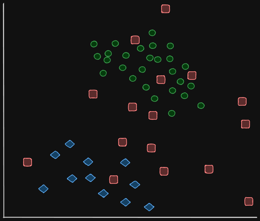
We have three different classifications here. As you can see though, they’re pretty intermingled, and it’s difficult in some areas what we’d classify each as. Now, let’s introduce two new shapes; a triangle and a pentagon. Then, we can draw lines to the nearest shapes to help us classify. Let’s use three;
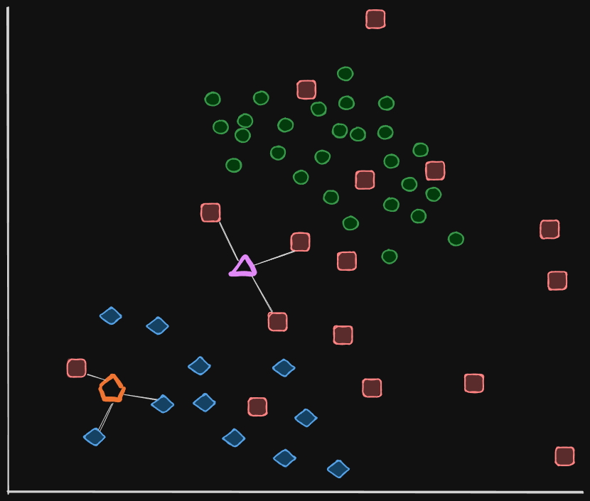
Now we can make our classifications. The triangle belongs to the squares, since it’s a clear majority of all three squares. The pentagon belongs to the diamonds, with a 2 to 1 win over the squares. This was also an easy example because we’re able to graph it using only two dimensions, meaning it only has 2 features. It’s entirely possible to have more though. We can use KNN with our MNIST data set; in that case, it would be a vector of 784 elements for each of the pixels, with 60,000 training examples, or points in space. KNN is unfortunately pretty slow though, since it has to calculate all the distances in the set.
KNN also has an interesting effect when observing how the amount of data points and dimensions reflects on the models accuracy. If we provide the model with all of the available training data for our MNIST set, we would get close to 99% accuracy. As we decrease the amount of data, obviously it gets worse, but not all that bad. With only 60 samples, which may or may not even contain all of the digits available (likely not), you’ll get a whopping 66% accuracy. Pretty good, and way better than a random guess.
There’s also this odd phenomena with a data set so large; the curse of dimensionality. Basically, the more dimensions there are, the more samples needed for accurate readings. Fortunately, because of the makeup of our dataset, our points will likely be clustered together. 5’s look like 5’s, and so on, making our classification easier than other data sets. If you want an example of how hard it is to scale KNN to more complex images, the CIFAR-10 data set is comprised of 50,000 images of 10 different classifications (cars, animals, etc.). A model with all 50,000 images is only accurate 35.4% of the time. Not great.
Decision Trees
We did one of these in chapter one, so let’s expand on them a bit more here. Everything starts at a root node, and conditional yes or no questions await each branching path. This is repeated until a final node called a leaf node is found, containing a classification or a label for whatever is getting classified.
These types of decision trees are what we call deterministic, or stay the same every time upon input. This is often not the most reliable upon complex data, so the need for forests of trees arose. One step further, since each tree is deterministic and we don’t want just one of the same tree over and over again, came random forests, a foundational concept in machine learning. In this forest of decision trees, each one is randomly constructed of the basic conditional statements making up the original tree. Each random tree has pros and cons, but our inputs have a much higher chance of correct classification in this manner than before.
Seems like making trees random shouldn’t work, or at least shouldn’t give you the same answer every time. The reason why it does goes like this; bagging, random feature selection, and ensembling. We start with our training data, and continue to make trees using our data set along with tree-specific training sets created through that bagging process mentioned just above. It’s the process of creating a new dataset using random sampling with replacement (we might use it more than once, or never!).
Here’s a basic example; we start with $[5, 9, 3, 4, 1, 2]$. Then, we start to make variations of this dataset, like;
- $[3, 4, 4, 9, 5, 5]$
- $[1, 9, 5, 2, 2, 1]$
- $[2, 2, 2, 9, 3, 5]$
We also call these bootstrapped data. In our case, we want to bootstrap our dataset for each randomly generated decision tree. This leads to the next step; training the tree on a randomly selected set of features. Every single tree in the random forest is trained using a bootstrapped version of your data, using only a subset of that data. If you understand that, you’re golden.
Onto the last part; using the tree by creating an ensemble of the answers provided by each tree. Each tree is going to spit out a value (more often then not, it won’t be understandable by a human) that represents a classification. All trees come together to do a majority-wins-type situation, meaning the more trees classify a label, that label will be chosen.
Support Vector Machines
Saving the best and most complex for last, support vector machines are not only math intensive, but are also definition intensive. Let’s start by laying out some groundwork; a visualization we can use for more clarity.
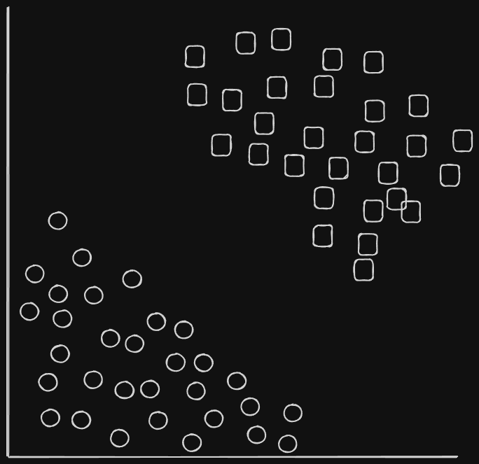
In the above example, we can very humanly see that each category is clearly separated; circles and squares. If we wanted to draw a line that separated each classification into it’s own designated space where each new entry would be classified correctly, where would that line go? If it’s too close to either category, you run the risk of miss-categorizing a potential circle or square.
Ideally, you probably want the line an equal distance furthest away from each group. This brings us to our first definition; margins. SVM’s goal is to maximize the margin between our classifications, or the widest separation between classes. For the above example, we can draw a line at the maximum margin;
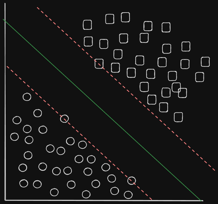
We have three lines drawn. The red dotted lines are the maximum boundaries, and the green line is the output of the SVM identifying the maximum distance between each margin. This is essentially what a SVM’s objective is. We have some more aspects of this we should learn about before we move on however, and that’s how these margins and separating lines are actually found.
First up; notice how in our boundaries, our line crosses through some points. These are called support vectors, and make up the SV-part of SVM. These are found using an optimization algorithm, which try to find the best solution given some input criteria. In our case, we’re trying to find boundaries, so our optimization algorithm should be attempting to find these values.
The last vocabulary term for this section is that of a kernel- not the popcorn type, but the mathematical type. In this context, kernel refers to the method your SVM uses it’s feature vectors. Using our above example as a base, that would be a linear kernel, since it uses the training data as is. There are other types, especially if the relationship between your vectors is unclear. The kernel will transform your feature vector into a different representation, likely not as human-readable.
More generally, machine learning engineers have been aiming at minimizing the features needed by a given model. This process of finding the right amount of feature vectors is also called feature selection or is sometimes referred to as dimensionality reduction. Think of the kernel is SVM as a type of feature selection. The features chosen reflects the effectiveness of the model. In these earlier models we often have to chose what features mean the most to us and make the most sense. This doesn’t always work, which is why as machine learning advanced, engineers will often “let the data speak for itself.”
Another term we might use for these “magic values” are called hyperparameters. SVM’s might have one or more depending on the kernel used, and neural networks can have many. Even with more parameters, the neural networks can often be thought of as easier to use, due to the sheer amount of data neural networks take advantage of and the amount of non-human interpolating done by the model.
One last point to touch on exclusively about SVM’s, is that they’re binary classifiers, meaning it’s going to be one or the other. But what if we have multiple different types of classes to distinguish from? One method engineers use it to create a SVM for each classification, and training each SVM to correctly identify one of each. Whenever an identification is made, the SVM also passes in a metric, or a unit of confidence. Given a new input, it’s fed to each SVM and the result with the highest metric is the correct classification.
Models in Use
So we just learned three brand new types of models. How do they actually fair in the real world? Well, let’s test them out. Again, all of these tests are coming directly from the text, so feel free to get more detailed insight there.
For the next test, we’re going to use a dataset of dinosaur footprints. More specifically, we have a little over 1600 images of either Theropod footprints or Ornithischian footprints. Just over 1300 will be used in our training, and over 300 will be left out for our testing. We’re going to train six models;
- Nearest Neighbor (For K = 1, 3, 7)
- Random Forest with 300 trees
- Linear SVM
- Radial Basis Function SVM
Here are the results;
| Model | ACC | MCC | Train | Test |
|---|---|---|---|---|
| RF300 | 83.3 | 0.65 | 1.5823 | 0.0399 |
| RBF SVM | 82.4 | 0.64 | 0.9296 | 0.2579 |
| 7-NN | 80.0 | 0.58 | 0.0004 | 0.0412 |
| 3-NN | 77.6 | 0.54 | 0.0005 | 0.0437 |
| 1-NN | 76.1 | 0.50 | 0.0004 | 0.0395 |
| Linear SVM | 70.7 | 0.41 | 2.8165 | 0.0007 |
Obviously, the model column refers to which model is being used. The ACC column is our models accuracy, or the result of the models confusion matrix. The matrix for reference looks something like this;
| Ornithischian | Theropod | |
|---|---|---|
| Ornithischian | TN | FP |
| Theropod | FN | TP |
Remember, we want to increase the number of TN or True Negatives for the Ornithischian, and the number of TP or True Positives for Theropods. We’ll get either a 0 for Ornithischian or a 1 for Theropod. Going back, the Random Forest was the most accurate with correctly labeling 83% of test images. We get this number by adding up TP and TN and dividing by the sum of all four outputs.
MCC, or Matthews correlation coefficient, works a bit differently but also uses the four numbers of our confusion matrix. It’s also thought of to be a better identifier of a model’s usefulness than it’s accuracy. This time, the range is from -1 to 1. 1 means no mistakes, and -1 is perfectly wrong, meaning you should probably flip your output classifiers and get a perfect 1.
We also have to take a look at Train and Test times. Each time is how long it took each model to perform each task; training our nearest neighbor models took milliseconds for example, since again the training is the data. We can also make inferences like how short it is to train certain models like KNN but take longer to use, or how longer linear SVM is to train compared to radial.
The biggest takeaways from a test like this is an expected understanding of performance for when we take a look at the more advanced neural networks of today, and just how useful these models can be regardless of advancements. In the paper this dataset originated from, the actual paleontologists were only correct 57% of the time, which is easily beaten by nearly all of the models presented and tested.
Chapter Summary
To reiterate, these models don’t really fall into either category of symbolic or connectionist. They don’t really use any logical rules the same way symbolic AI does, and they aren’t made up of smaller modules that learn from each other, which means they aren’t connectionist either. The best way to consider these models as models that produce functions that fit our data. The function changes depending on the model used, but they almost all produce one (except KNN).
Next: Chapter 4