And Away We Go: An AI Overview

Consider this the master chapter for all basic AI definitions. Everything following this chapter will build off of the points brought up in this chapter. Some foundational stuff right here.

Again, we should start at the most basic; Artificial Intelligence is the process of training a machine or computer to act like an intelligent human being. This original terminology was first used by John McCarthy in the 1950’s!

Computers are programmed to accomplish tasks, or a program, which is usually encompasses some algorithm that controls to logic of said program. Imagine you own a burger truck, and you have your own special ketchup only you know the ingredients to. That recipe is the algorithm, the construction of the burger sauce is the program, and the workers who make it all happen is the machine (or in this case, model). The workers don’t need to fully understand the recipe or even why they are doing whatever they’re doing; that understanding is held usually only by the programmer, or in this case you as the owner of the sauce recipe.

This is the way it’s be done for years; programmers will write some code containing an algorithm, the machine will perform the tasks without even considering why it’s doing it in the first place. If we had to give anyone credit, it would fall likely onto Alan Turing in the 30’s or Charles Babbage (Technically Lovelace also, but we’ll get more details later in chapter 2).

Terminology: AI, Machine Learning, and Deep Learning

When beginning, most people will use the above three terms interchangeably. On a surface level, they’re not wrong, but they are certainly over simplifying it. The real relationship between all these terms looks something more like this;

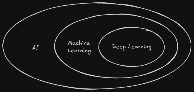
Deep learning is a sub-field of machine learning, which is in itself a sub field of artificial intelligence. There’s a lot going on in the first circle; we’ll call this the old days. In the old days of AI, approaches before 1950, are going to be generally ignored by this text. Instead, we’ll flesh out the other two terms.

When we refer to machine learning, we’re creating our models using existing, quantifiable data. When we say model, we’re talking about a device that takes in input and generates some output. Obviously, this input and output is meaningful in some regard, giving us some information that can be used in real time. Using that input data, we can use the known data to produce output for instances where we don’t know enough about our data. Deep learning on the other hand uses huge models to accomplish tasks otherwise not computable. If the above two terms are confusing, don’t stress; we’ll get there.

The terminology even by professionals is largely interchangeable, but you should be able to distinguish between the three. The best way is to think of deep learning as a large neural network (we’ll get there I promise), machine learning as models trained by data, and AI as a catchall.

What is a Model?

Most commonly associated with machine learning, the model is again that intangible entity that takes in input and produces an output. Sometimes the output is a word or phrase, other times it’s a numerical value. These are most often predictions. For example, let’s say we wanted to build a model that can determine if a given image is of a dog or not. It can either output “dog” or “not dog”, or even a percentage of how confident the model is that the image contains a dog. One of the first uses we’ll get to is with Linear Regression, where we’ll predict the pricing of houses based on some unique features.

To continue with definitions, every model has a set of parameters that determine the output from the model. We train a model by setting these parameters accordingly until we get some desirable result. Now, the most confusing part of the training process is that not only do we train on input, but also output. Basically, we are telling our model given this set of inputs, this is what the output should look like. This prepares the model to handle input data where we don’t always have all the input information we gathered in our training data.

Using our Linear Regression example, say we have the following table of data;

Rooms	Year Built	Square Feet	Price
3	1997	4000	180,000
4	2007	6000	380,000
2	2003	4500	190,000
5	2024	10000	780,000

If our goal was to make a house price predictor, the first 3 columns (Rooms, Year Built, and Square Feet) would be our input, while the Price would be our output. Now, given we get in a new home, with 4 bedrooms, built in the year 2018, and 7500 square feet of space, how much would that cost? Well, given the previous 4 pieces of data, we could design a model that uses all of the available features to make a mathematical approximation.

The “training” portion of a model actually uses little to no programming; the programming, remember, is the set of instructions to run on our data. Often, we don’t know what algorithm would best suit for desirable output. One thing we have to note here is the already apparent use of bias; if I don’t like the results of my model, can I mess around with my training data until the results suit my agenda? Absolutely. A quote from a British mathematician, “Models are always wrong, but some are useful.”

The algorithm for machine learning follows these four steps;

Collect training data (both input and output)
Select type of model to train
Train model and adjust parameters if output is incorrect
Repeat step 3 until satisfied with performance
Use the model

The method we just outlined is called supervised learning, since we know all of the data we are training our model on (sometimes refereed to as labeled data) and are actively making adjustments in the process of training it.

Setosa vs. Versicolor

One of the most popular examples of machine learning, we’re given a dataset containing measurements of an Iris flower. The different types of Iris’ can be classified based on these measurements, and we can define them as either setosa or a versicolor. These are split on the flower petal’s length and width. Dating back all the way to the 1930’s, this model takes in two inputs and returns one of two outputs, making that model a binary model. If there were more than two species, it would be a multiclass model.

Math Terminology

Math sucks. At least to some people it does; unfortunately it’s a key element to computer science as a whole and will directly help us understand AI. Models will almost always use either vectors or matrices. If you want a more detailed overview of some linear algebra, you can visit this note. Here’s the basic breakdown;

Vector: A set of numbers as a single entity
- Ex. Using our iris flower representation; {4.5, 2.3, 1.3, 0.3}
  - Sepal length and width, and petal length and width
- Dimensions defined by amount of numbers
Matrix: Two-dimensional array of numbers

We’re going to run into these two structures all the time. For example, our iris flower data set is not just a vector, but a matrix of all the iris flowers, with each row being another iris.

More Model Definitions

The name we give to our input data in machine learning is features; our Iris dataset has two features, petal length and width. A single entry is known as a sample, or a feature vector. Again, we’re working with a binary model, so in our case we’re going to get an output of a number of confidence it belongs to a flower species (If confident it’s not, that indicates it’s the other species!).

Now, even though collecting data can be a ton of work on it’s own, we can’t just give a model some data and assume it’s going to work all of the time. Quite often, because we don’t always understand what decisions a computer decides to make in split micro-second instants, the first time you run a model it will be off. One way to ensure we have some room to test is by using only a percentage of our dataset for training initially, then using the rest for post set-up testing. Something like a 80/20 split makes sense.

The machine learning term for what we were just talking about is optimization, when engineers fit the data compactly so patterns can be easily recognized. What you really want out to do with your model is have it generalize, or have the model understand the general characteristics of your training set so your test set has good generalization abilities. Confusing, so let’s take a look at this using our iris flowers;

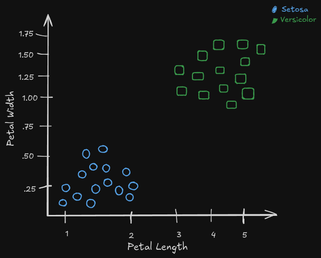
Taking a look at our scatter plot, we should see a clear pattern; all of the similar flower species are grouped together based on these two features. The special type of model we want to build in this instance is called a classifier, since we want to be our model to tell us which class any new entries fall into.

Not only is it a classifier, but we also have to end up choosing a type of model. We could go for a decision tree, which is like our computer playing 20 questions with each new entry. But, since our features are so basic and we only have two classifications, we can just observe out data set and make a single question our classifier; if the petal length is less than 2.5 cm, it’s a class 0 or setosa. Otherwise, it’s a class 1 or versacolor.

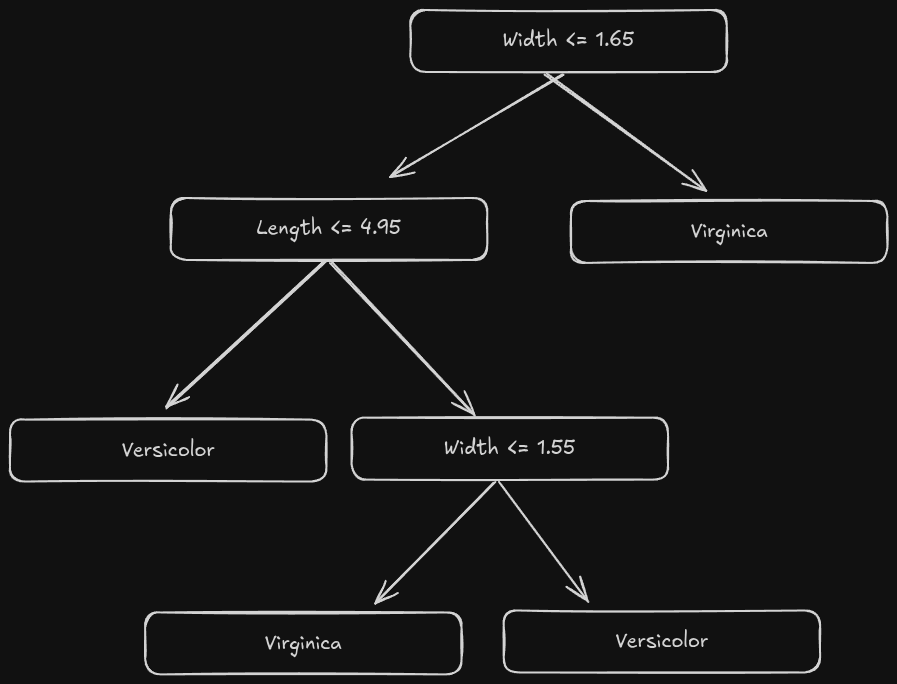
For now, this works. If we throw in more data, and it happens to stay correct, then we can confidently say we’ve built a properly working classifier. One simple way to disrupt this harmony is to throw in another species; virginica. All of a sudden, based on petal length and width, our classifier would become unusable with data points all over the place. It’s in this instance we want to go for a decision tree, like the following;

The model we made is good for a very specific purpose. In the grand scheme of things, it’s not so complex. One way we can judge complexity is through the ability to classify under more broad conditions. Going back to our dog classifier. Say we train our model on dogs and lizards. If we introduce something that looks like a dog, like maybe a wolf, will our model be able to tell the difference? Probably not, because our model has no prior experience with wolves, and they look an awful lot like a regular dog to most people. If our model can work well “in the wild”, we’ve got a pretty strong model.

Another example we can refer too is the MNIST dataset, a collection of small integer numbers used to train neural networks on identifying these integers. Since we’re identifying images, and we know the images are 28x28 pixels, that makes each image have 784 features (or dimensions). This is obviously a lot more than the 2 features we just looked at, but machine learning can handle it no problem. This is such a simple example, anybody can use open source toolkits (like we’re going too later on in the course) to run this themselves.

For now, let’s say we want our model to correctly identify 0, 1, 3, and 9. We’ve got a ton of samples; nearly 25,000 images, with around 6,000 for each of our 4 digits. We’re going to leave out about 4,000 images, one thousand for each digit. We can make a confusion matrix to show this empirical relationship;

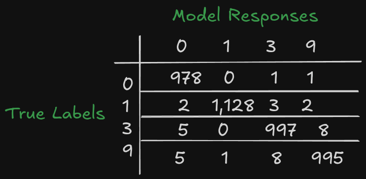
Each row is the actual number label, with each column being the models response. For example; for the digit 0, the model responded correctly 978 times, and incorrectly label a single 0 as a 3, and another as a 9. We can use the diagonal (or where each corresponding matching numbers meet) to get a quick look at whether our data is being read correctly; the diagonal should contain high numbers, while the off diagonal contain small, relatively forgettable numbers.

Quantified out, this is a 99% approval rate. Pretty good! Except, our issue comes from the inclusion of any other digit. Say we ask it to give us a 4; how would our model respond? The text model get’s this as it’s answer for 4’s:

0	1	3	9
48	9	8	917

And then again for 7’s:

0	1	3	9
19	20	227	762

First off, notice how our models responses don’t change even though we’ve added another type of input. Because our model was never trained to recognize 4’s or 7’s, it will never respond with those options. It will try to fit whatever new input into one of the already existing classifications.

Some more definitions for you, if this chapter hasn’t been dense enough. We can break down the above example into two terms; interpolation and extrapolation. Interpolation will respond with known output, and extrapolation will push further than what it’s been trained on. Let’s use an example; say when we trained our models on 0’s, all the images were of 0’s in neat and straight-up manner. If we were to introduce a slanted or tilted 0, the model will have to interpolate to get the classification correct. If we introduced a 0 with a slash through it (sometimes used to denote between 0 and capital O) the model will have to extrapolate, since it’s never been seen and distinguishable enough from a basic tilt or lean.

Another example we can observe; population between 1950 and 1970. Observe the following graph;

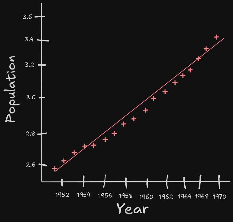
This is yet another version of machine learning we will come across this year, but for now I want to focus on those two vocab words we just learned. Since we have the dataset from 1950 to 1970, our model interpolates what the expected population should be, which is compared directly to our actual (the line of best fit). If we wanted to our model to predict the population before 1950 or 1970, it would have to extrapolate.

If we actually look at the population growth up to today, the above line of best fit is actually quite bad. As the years pass, the expected versus actual value continue to widen, meaning we would need to rerun our model with all of the available data to get a new line of best fit that’s more accurate. We call this process curve fitting, which is like a younger cousin to machine learning. In general, we want to avoid extrapolating, and should always prefer interpolating.

Cautionary Tales

With great power, comes great responsibility. Again, a point I will stress over and over again, your models have no real thought behind them. A great story from the text; a machine learning researcher tried to uncover reasoning behind neural networks and why models behave the way they do. For his training set, he tried to create a model that tells the difference between wolves and huskies (pretty similar looking animals). The model was pretty good at it’s job! It was accurate and that’s all that matters, right?

After taking a closer look at how the model made it’s decisions, this assumption becomes moot. Turns out, the training data of all the wolves included snow in the background, while the huskies did not. The model was only deciding it a wolf was a wolf if the picture had snow in the background. Without questioning the means and methods behind a model, one can very quickly accept incorrect information as valid. In other cases, sometimes models pick up on features non-perceivable to the human eye, making understanding near impossible.

Another phrase to keep in mind when observing model behavior is “Correlation does not imply causation.” Essentially, just because the rooster crows before the sun comes up, does not mean the sun rises purely because of the rooster. Both happen at the same time; they correlate but do not directly affect one another. Our models might learn about data concerning our subjects, but our models will never truly understand our subjects. This has lead to huge issues; Google had a huge issue post release of their AI trained photos app in 2015. The best way to avoid issues like these is to use diverse training data.

Going back to our numeric example, we want our model to be able to accept any kind of representation that could be considered a digit. That means some 0’s that are normal, some slanted, some with slashes through it, etc. Let’s make it a little more basic; instead of identifying digits, all it needs to do is tell us if it’s a 9 or not. Again, using the same dataset as before, without the inclusion of 4 or 7. we went from a multiclass model to a binary model Running this would give you a pretty good result;

	Not 9	9
Not 9	9754	23
9	38	1362

Some things we can observe from this;

The new model has 23 false positives, or where the model said a digit was a 9 when it actually wasn’t
The model has 38 false negatives, or when the model said a digit wasn’t 9 when it actually was

We ideally want a model with no false positives or negatives, but often that is impossible. Usually, it’s better to prioritize minimizing false negatives; think of a medical use. If testing for cancer, a false positive will warrant a further look until you see there is no cancer. However, a false negative is a missed catch, meaning that person now does not know they have cancer when it was incorrectly caught. It’s always going to be depend on what the model is being used for.

Chapter Summary

Models are trained on datasets, usually made up of many matrices of input and output data.
The best types of models are trained on a wide variety of data, in order to interpolate data rather than extrapolate
Bias will show in models; if the training data is biased, so is the model
Models are always wrong, some are useful

Chapter Resources

Next: Chapter 2

How AI Works - Chapter 1