Introduction to Algorithms - Chapter 2
Getting Sorted
This chapter is meant to familiarize yourself with the framework used throughout the book.
2.1 Insertion Sort
Solves a sorting problem (obviously).
The numbers to be sorted are known as keys.
The input comes in the form of an array with n elements.
A reason to sort is often because those keys are associated with other data, Satellite data.
Key + Satellite = Record
We can think of a spreadsheet, with student records having many pieces of data. Any piece can be the key; whatever the key is, is how the record is sorted.
They offer the code into pseudocode, and I turned it into Python.
Pseudocode:
Where A is an array and n is the # of values.
Insertion-Sort(A, n)
for i = 2 to n-
`key = A[i]` -
`j = i - 1` -
`while j > 0 and A[j] > key` -
`A[j+1] = A[j]` -
`j = j - 1` -
`A[j+1] = key`
def insertion_sort(nums:list) -> list:
	"""Sort a list using insertion-sort algorithm."""
    max_len = len(nums)
    for i in range(1, max_len):
        key = nums[i]
        j = i - 1
        while j >= 0 and nums[j] > key:
            nums[j + 1] = nums[j]
            j -= 1
        nums[j+1] = key
    return nums

number_list = [6, 3, 8, 1, 10, 2, 1]

print(insertion_sort(number_list))
Let’s think of this like a deck of cards. In the example, at the beginning of each iteration of our for loop, indexed by i, the subarray consisting of elements A[1:i-1] constitutes the currently sorted hand, and the remaining sub array A[i+1:n] corresponds to the pile of cards still on the table.
We state these properties of A[1:i-1] formally as a loop invariant:
At the start of each iteration of the **for** loop, of lines 1 - 8, the subarray of `A[1:i-1]` consists of the elements originally in `A[1:i-1]`, but in sorted order.
Loop invariants help us understand why an algorithm is correct. We need to show three things:
- Initialization: It’s true prior to the first iteration of the loop.
- Maintenance: If it was true before, it remains true before the next iteration.
- Termination: The loop terminates, and when it does, the invariant - usually along with the reason that the loop was terminated = gives us a useful property that helps show that the algorithm is correct.
When the first two hold true, the loop invariant is true prior to every iteration of the loop.
A loop invariant proof is a form of mathematical induction (prove a base case, then an inductive step).
The third property might be the most important since it proves correctness.
Unlike mathematical induction, where the inductive step infinitely, in the loop invariant the “induction” stops when the loop terminates.
Let’s review how the induction proves each of the three points:
- Initialization: We start by showing it holds before the loop begins, when
iis 2, since logically there is only one element that has to be sorted (obviously). - Maintenance: Using the logic of the for loop, and that it increments up by one each turn, we preserve the loop invariant (we’ll talk about the while loop later).
- Termination: Due to the condition,
ibeing greater thannori = n + 1, it will end, and it hasA[1:n]sorted, so the algorithm holds correct.
Some Pseudocode Conventions:
- Indentation indicates block structure.
- Looping constructs while, for, repeat-until, and if-else work just like they do in C, C++, Java, and Python.
- The for loop’s counter retains the value that broke the loops bound.
- // denotes a comment.
- Variables
i,j,key, etc. are always local unless specified. - In Python specifically,
for\ i = 1\ to\ nis equivalent tofor i in range(1, n+1).- Also in Python, the loop counter retains
n, notn+1because lists may contain a non-numeric.
- Also in Python, the loop counter retains
- Indexing lists/arrays works similarly to Python, except this book uses 1-origin over 0-origin slicing
:indicates a subarray. - Data objects will often exist, and it’s attributes are access via dot method.
- The book treats variable representing an array or object as a pointer to the data representing the array/object.
- If you set
y=x, and changex.fto 3,y.fis also 3 now.
- If you set
- Parameters are passed by value, instead of by reference.
- The procedure receives its own copy of the parameters, and if it assigns a value to a parameter, the change is not seen by the calling procedure.
- Return statements return control back to the point of call & often can return values. Often, the book will contain a few return values, which is unconventional for most languages.
- Short-circuiting is when you use
andandorto bypass quick conditionals.- With
and, ifxandy, andx=false,yis not checked. - With
or, ifxandy, andx=false,yhas to be checked.
- With
- Error is an error.
Exercises 2.1
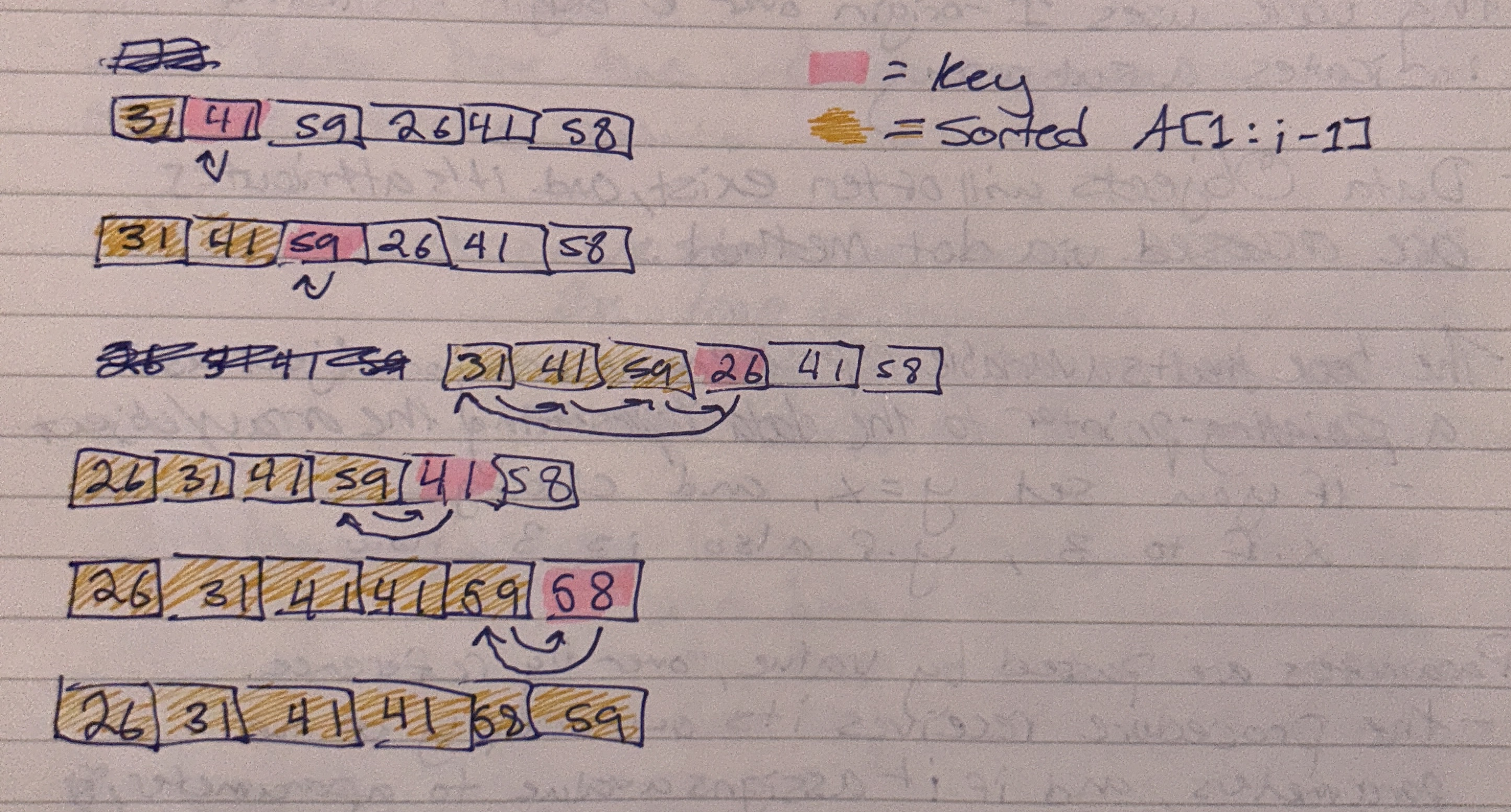
- Using Figure 2.2 (insertion sort diagram), illustrate the operation of insertion sort on an array containing the sequence (31, 41, 59, 26, 41, 58).
- Consider the following procedure, Sum-Array. It computes the sum of the
nnumbers in arrayA[1:n]. State a loop invariant for this procedure, and use it’s initialization, maintenance, and termination properties to show that the Sum-Array procedure returns the sum of numbers inA[1:n].
Sum-Array(A, n)
sum = 0for i = 1 to n-
`sum = sum + A[i]` return sum
Invariant: After the initial start of each iteration of the for loop of lines 2 & 3, the variable sum sill contain the running sum of A[1:i-1].
Initialization: Sum is 0, then after the first loop, always equal to A[1:i-1].
Maintenance: For loop moves from first element to n (max size).
Termination: Returns sum after loop completes.
- Rewrite the insertion-sort procedure to sort into decreasing order instead of increasing order.
def insertion_sort(nums:list) -> list:
	"""Just change > to < keys"""
    max_len = len(nums)
    for i in range(1, max_len):
        key = nums[i]
        j = i - 1
        while j >= 0 and nums[j] < key:
            nums[j + 1] = nums[j]
            j -= 1
        nums[j+1] = key
    return nums
7/31/24
- Consider the following searching problem, and write pseudocode for linear search, which scans through the array from beginning to end, looking for
x. Using a loop invariant, prove that your algorithm is correct.
Input: A sequence of n numbers (a_1,a_2,...,a_n) stored in an array A[1:n] and a value, x.
Output: An index i such that x equals A[i] or the special value NIL is x does not appear in A.
Linear-Sort(A, x)
n = length of Afor i = 1 to n-
`if A[i] = x` -
`return i` return NIL
Loop Invariant: For each iteration of the for loop on lines 2, 3, and 4, each value of A is compared to x. If any value is, the index i is returned. If no value is found, NIL is returned.
Initialization: n creates our bound, so we don’t go over and get an index error.
Maintenance: Unless the condition is met, no changes are made, except for loop iteration.
Termination: The last command is returning NIL, ensuring closure.
2.2 Analyzing Algorithms
Analysis is the method of predicting the output of an algorithm based on numerous factors. Energy, time, space, etc.
In order to analyze properly, you need to first understand the environment, limitations & specifications, etc.
The book uses the Random Access Memory (RAM) method:
- Everything is stored in the same fashion (think of arrays, allocating the same space for each element).
- Each command requires the same time (instruction or data processing).
- Each instruction happens one after another with no congruency
- Some pre-built instructions:
- Arithmetic (add, subtract, multiply, etc.)
- Data movement (load, copy, store)
- Control (conditional/unconditional branch, return)
- Data types are:
- Integers (Booleans are just integer checks for
0=falseand1=true) - Floats
- Characters
- Integers (Booleans are just integer checks for
Analyzing Insertion Sort
You could run it on your computer given the code above. You could time it, but that wouldn’t tell you much.
The reason is that every computer environment is different, along with different input factors that make comparing directly difficult.
Instead, we can analyze the algorithm used itself, or, how long each instruction takes to complete.
We’ll do this in two steps:
- Come up with a formula for running time.
- Use the important parts of the formula in an easy to read notation.
8/10/2024
Likewise, there are two distinct factors we need to keep in mind: Running time and input size. They will affect our algorithm in different ways.
Input Size as a notation is dependent on the problem. In some, like sorting, notation is the number of items in the input. For others, like multiplication, notation is the number of bits needed to represent output.
Running time is the number of instructions/data accesses executed.
- In the following examples, so we can understand the execution of a line (since lines might take longer than others) that each execution of the
kth line takesC_ktime, whereC_kis some constant.
Let’s examine the Insertion sort method line by line:
Insertion-Sort(A, n)                  Cost             Times
1. for i = 2 to n                      C1                n
2.   key = A[i]                        C2                n-1
3.   // Insert ''                       0                n-1
4.   j = i - 1                         C4                n-1
5.   while j > 0 and A[j] > key        C5       Summation(i=2, n) * ti
6.     A[j + 1] = A[j]                 C6    Summation(i=2, n) * ti - 1
7.     j = j - 1                       C7    Summation(i=2, n) * ti - 1
8.   A[j + 1] = key                    C8                n-1
We can turn this into a formula, for which we can say:
T(n) = C_1n+C_2(n-1)+C_4(n-1)+C_5 \sum_{i=2}^{n}*t_i+
C_6 \sum_{i=2}^{n}*(t_i-1)+C_7 \sum_{i=2}^{n}*(t_i-1)+C_8(n-1)
In the best-case scenario, line 5 will never activate, and it becomes an entirely different formula:
T(n)=C_1n+C_2(n-1)+C_4(n-1)+C_5(n-1)+C_8(n-1)
Which becomes:
T(n) = (C_1+C_2+C_4+C_5+C_8)n - (C_2+C_4+C_5+C_8)
From this equation, we can say the running time is a linear function of n, (an+b).
The best-case scenario is nice, but likely this will not be the case. Often in the world, we wouldn’t need sorting algorithms if they were already sorted before we got there.
We need to account often for the worst-case scenario.
For insertion sort’s case, the worse case would be if every number were in reverse order.
- In this scenario, our while loop will have to compare each element with every number in the sorted array
A[1:i-1], sot_i = i \ for \ i=2,3,...,n. - This changes our notation slightly:
\sum_{i=2}^{n}*\ ibecomes(\sum_{i=1}^{n} * \ i) - 1- We can also use Appendix A, to simplify it even further:
(\sum_{i=1}^{n} * \ i) - 1becomes(n(n+1)/2) - 1
- We can also keep simplifying our other terms
\sum_{i=2}^{n}*\ i-1becomes\sum_{i=1}^{n-1} * \ ibecomesn(n-1)/2
Our worst case insertion sort running time formula becomes:
T(n) = C_1n+C_2(n-1)+C_4(n-1)+C_5((n(n+1)/2) - 1)+
C_6(n(n-1)/2)+C_7(n(n-1)/2)+C_8(n-1)
and can be simplified even further:
T(n) = ((C_5/2) + (C_6/2) + (C_7/2))n^2 + (C_1+C_2+C_4+(C_5/2)-(C_6/2)
-(C_7/2)+C_8)n-(C_2+C_4+C_5+C_8)
From the above formula, we can express our worst-case running time as an^2+bn+c for constants a, b, c. Running time is a quadratic function of n.
Worst Case & Average Case Analysis
3 reasons to consider worst case over best case:
- It acts as an upper-bound (the algorithm will never take longer than worst-case).
- For some algorithms, worst-case occurs often.
- The “Average” case is often as bad as worst-case.
Order of Growth
We used levels of abstraction already (C_k, an+b ignoring C_k, etc.)
We can abstract even further. It’s the rate of growth/order of growth we can actually analyze our running times by.
At large values of n, the low-cost terms mean almost nothing, so we can ignore them. We can also ignore constants, since they’re less relevant for larger values of n.
For insertion sort’s worst case an^2+bn+c, we drop the bn+c since they’re a lower term, and drop the constant a.
Theta, \Theta, can represent this:
- Worst-case running time of insertion sort is
\Theta(n^2).
For right now, the definition is rather loos. We’ll get a more precisie definition in the next Chapter.
An algorithm is known to be more efficient than another if it has a lower order of growth
Exercises 2.2
- Express the function
n^3/1000+100n^2-100n+3in terms of\Theta-notation
For \Theta-notation, since we can drop the lower terms & constant from the higest term, \Theta(n^3) is the notation.
- Consider sorting
nnumbers stored in arrayA[1:n]by first finding the smallest elements ofA[1:n]and exchanging it with the element inA[1]. Then, find the smallest element ofA[2:n], and exchange it withA[2]. Then, find the smallest element ofA[3:n], and exchange it withA[3]. Continue in this manner for the firstn-1elements ofA. Write pseudocode for this algorithm, which is known as selection sort. What loop invariant does this algorithm maintain? Why does it need to run for only the firstn-1elements, rather than for allnelements? Give the worst-case running time of selection sort in\Theta-notation. Is the best case any better?
Selection-Sort(A, n)                  Cost             Times
1. for i = 1 to n-1                    C1               n-1
2.   min_value = A[i]                  C2               n-1
3.   for j = i + 1 to n                C3   Summation(i=0,n-2)*(n-i-1)
                                            ^ this becomes (n(n-1)/2)
4.     if A[j] < min_value             C4            (n(n-1)/2)
5.       min_value, A[j] = A[j], min_value   C5      (n(n-1)/2)
6.   A[i] = min_value                  C6                n-1
I was having trouble getting started with how to view the times each line would run, so I asked ChatGPT for help. It definitely helped put the Times category into perspective.
\Theta(n^2) is our simplified worst-case running time.
Loop Invariant: For each iteration of the for loop on lines 3-5, the first element up to the last will be compared and switched with the larger number until the entire list is sorted.
UPDATE: After comparing our answers, it appears that the structure for these answers follow a similar pattern:
- State the current status: (there algo is different, so doesn’t directly apply) “…at the start of each iteration of the outer for loop, the sub array
A[1:i-1]consists of thei-1smallest elements in the arrayA[1:n]” - After, then state what changes will be made for proof: “After the first
n-1elements, the sub arrayA[1:n-1]contains the smallestn-1elements, sorted, and therefore elementA[n]must be the largest element.”
Initialization: n is the length of A, and min_value is always equal to i.
Maintenance: First for loop moves through the whole list A[1:n-1], while the second loop only goes from A[j:n].
Termination: We use up to n-1 for the first loop, ensuring we never loop out of index/range, and stop.
The best case scenario is not much better, since it also has a running time of \Theta(n^2). It just doesn’t have to make the switch, but it still has to make the comparison.
- Consider linear search again (Exercise 2.1 #4). How many elements of the input array need to be checked on the average, assuming that the element being searched for is equally likely to be any element in the array? How about in the worst-case? Give
\Theta-notation for average and worst case.
In the average case, the value to be found, x, could be any, but has a normal distribution of being in the middle. We could say, \Theta(n/2).
In the worst case, we would assume x is A[n], the last element in the array. The being said, \Theta(n) would be it’s notation.
- How can you modify any sorting algorithm to have a good best-case running time?
I guessed, but by possibly eliminating any unnecessary comparisons?
UPDATE: You can edit the algorithm so it checks if the input array is already sorted before performing any operations. That way if it is, no steps are made.
8/26/2024
2.3 Designing Algorithms
Insertion Sort uses an incremental approach. We’re going to see a few that use other methods.
Divide and Conquer is a method we’ll look more closely at in chapter 4, but it’s importantly another methodology to use rather than an incremental approach.
Divide and Conquer Method
Recursion and Divide and Conquer go hand & hand. Recursion is when an algorithm will call itself one or more times to solve some problem.
Divide and Conquer problems will usually recursively break down the large problem into smaller sub problems to solve.
There are two usual cases for Divide and Conquer:
- Small problems don’t need recursion, we just solve them (we’re going to call this the base case).
- Large Problems work in this order:
- Divide the problem into smaller sub problems
- Conquer the sub problem recursively.
- Combine the sub problem solutions to solve the original solution
Merge sort follows Divide and Conquer methodology, starting with A[1:n]:
- Divide the sub-array
A[p:r]to be sorted into two adjacent sub arrays, each half the size- To do this, you can find the midpoint,
q, (Average ofpandr) and takeA[p:r]intoA[p:q]andA[q+1:r].
- To do this, you can find the midpoint,
- Conquer by sorting the two sub arrays using merge sort
- Combine by merging the sorted two sub arrays back into
A[p:r].
We say recursion ends, or “bottoms out”, reaching the base case, when the sorted sub array only has one element.
We can use a card example to understand the Merge Procedure:
- If you have a deck of cards, let’s say 52.
- In Merge Sort, you have
Merge(A,p,q,r), whereAis the deck of cards, andp,q,rare some indexes wherep<=q<r. We assume adjacent sub arrays. - In our example, our one 52 card stack becomes two 26 card stacks. (Merge also assumes each stack is sorted)
- We look at each top card and compare which of the two is smaller. Importantly, this is what we call the first step. The smaller goes to an output pule, and is replaced by another card. This is done until one card is left, which by default should be our highest order card.
- The best case is where since both sub stacks are sorted, only
n/2steps are taken. 26 steps, since there is no comparing the second pile. - The worst case is where you need to compare every card, so at most
nsteps. 52 steps (technically 51, since after 51 steps, one pile is empty). - Since we analyze algorithms for worst case, we could say the running time is
\Theta(n).
Let’s start by first laying out the pseudo code:
Merge(A, p, q, r)
1. nL = q - p + 1        // length of A[p:q]
2. nR = r -q         // length of A[q+1:r]
3. let L[0:nL-1] and R[0:nR-1]
4. for i = 0 to nL - 1      // copy A[p:q] into L[0:nL-1]
5.      L[i] = A[p+i]
6. for j = 0 to nR - 1     // copy A[q+1:r] into R[0:nL-1]
7.      R[i] = A[p+i]
8.