Dijkstra’s Algorithm

Dijkstra’s Algorithm calculates the shortest path on a weighted graph. Unlike Breadth-first search, every step we take has some cost associated with it that we have to take into account. Just like last chapter, we can use graphs to help us get a better understanding:

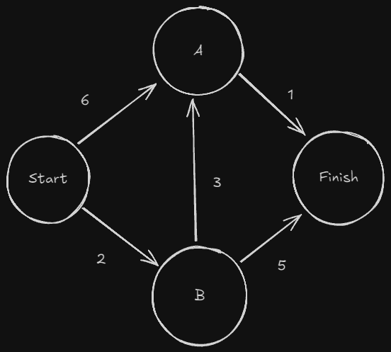
From what we know of BFS, we can assume it would probably return “Start -> A -> Finish” as the shortest path. without weights, that makes perfect sense. However, that has a cost of 7 (7 minutes). Isn’t there a cheaper way to get there? We’ll see in a second how Dijkstra’s algorithm calculates this for us.

Here is how it works;

Find the cheapest node

Node	Time
A	6
B	2
Finish	$\infty$
Since we haven’t reached Finish yet, we’ll leave it marked as $\infty$. We’ll see why soon. We have two options from Start, A or B. B is cheaper, so we start there.

Calculate how long it takes to get to the next nodes out-neighbor

Node	Time
A	5
B	2
Finish	7
3. Repeat, in this case A is the last node to check

Node	Time
A	5
B	2
Finish	6
The time in this scenario is our weight. Dijkstra’s algorithm only works on weighted graphs, and the weights cannot negative. If you an all positive weighted graph, Dijkstra’s algorithm could be useful.

Implementation

How could we try out the above example in Python? Once again, we can make use of hash tables, or in this case, dictionaries.

graph = {}
costs = {}
parents = {}

Here’s a visualization of how we can think about how to populate these dictionaries. We need to consider that we have to literally make the graph, so we should have an entry for each node, as well as keeping track of it’s out-neighbors and the cost associated…that’s a lot already. Not only do we need to keep track of the current and updated costs, but also the parents of each node.

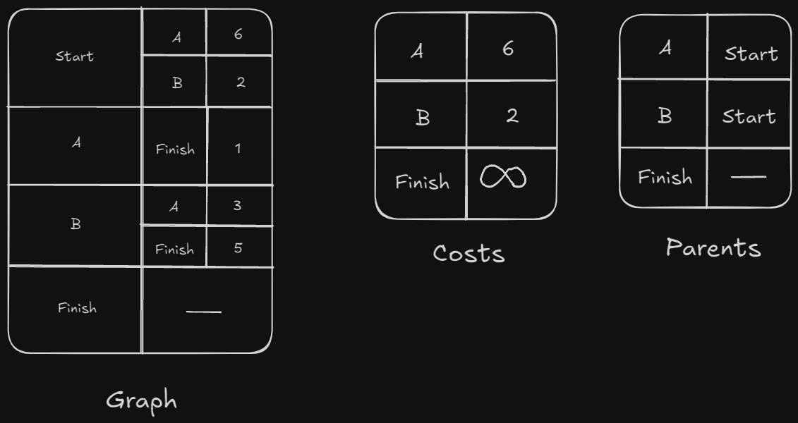
The best way to replicate this is actually with sub dictionaries:

graph['start'] = {}
graph['start']['A'] = 6
graph['start']['B'] = 2
...

For Costs, we can use the math module to help us out:

infinity = math.inf
costs = {}
costs['A'] = 6
costs['B'] = 2
costs['Finish'] = infinity

and for parents,

parents = {}
parents['A'] = 'Start'
parents['B'] = 'Start'
parents['Finish'] = None

Last but not least, we also need a set! Remember, sets cannot contain duplicates, which is going to help us in a second.

processed = set()

The logic for the algorithm is as follows:

Grab the cheapest node that is closest to the start
While we have nodes to process…
1. Update costs for it’s neighbors
2. If any neighbors’ costs were updated, update the parent as well
3. Mark this node as processed
4. Find the next cheapest node

node = find_lowest_cost_node(costs)
while node is not None:
	cost = costs[node]
	neighbors = graph[node]
	for n in neighbors.keys():
		new_cost = cost + neighbors[n]
		if costs[n] > new_cost:
			costs[n] = new_cost
			parents[n] = node
	processed.add(node)
	node = find_lowest_cost_node(costs)

There is a lot going on there. We should definitely take a walk through that in the debugger to really see behind the scenes how it works, step by step. There is one thing left out; the function called find_lowest_cost_node()!

def find_lowest_cost_node(costs):
	lowest_cost = math.inf
	lowest_cost_node = None
	for node in costs:
		cost = costs[node]
		if cost < lowest_cost and node not in processed:
			lowest_cost = cost
			lowest_cost_node = node
	return lowest_cost_node

Next: Chapter 10

Grokking Algorithms - Chapter 9

Dijkstra’s Algorithm

Implementation