Breadth-First Search

Graphs are the next data structure we are going to learn. Breadth-first search is the first graphing algorithm we’ll take a look at, and will give us the ability to find the shortest distance between two points.

There are many use cases for BFS:

• Spell checker
• Finding nearby doctors/hospitals
• Search engines

Graphs come in many different forms. One of the easiest ways to visualize is with locations:

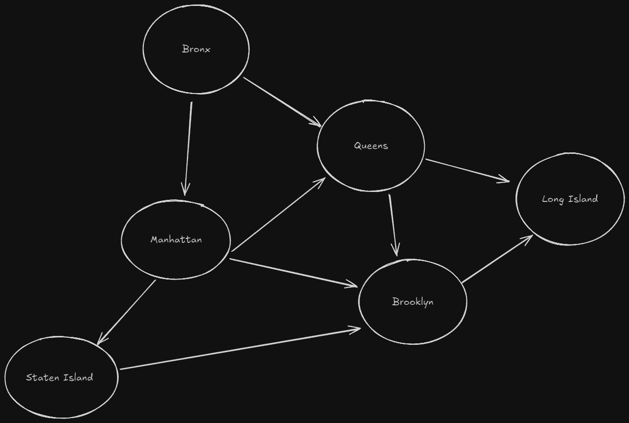
The arrows are only pointing in one direction, indicating this is a start to finish graph. We start in the Bronx, and want to end in Long Island. How many possible paths do we have there?

If you said 5, you would be correct! What BFS is going to do is move one step from the starting position, and keep incrementing until the finish node is reached. This is known as a shortest-path problem.

Graph Vocabulary

The graph itself is models the connections between entities. Each node represents another entity, and the edges are the lines between them representing the connections. The arrow facing determines whether that node is an out-neighbor or in-neighbor. In the above example, Brooklyn is an in-neighbor to Manhattan, and Manhattan is the out-neighbor or Brooklyn.

Using Breadth-First Search

Not only is it a search algorithm, it actually accomplishes two things, asking two questions;

1. Is there a path? (touching all nodes in the progress)
2. What is the shortest path between two points?

If we had a network of connections showing the people I know, and nodes for all the people they know, it would grow pretty quickly. Say I wanted to find someone who sells records, old vinyl. I would start with my connections, then check all of my connections’ connections, and so on until a record seller is found.

We can use BFS to solve this issue. It will see if we have a record seller in our own network, as well as our outer connections. It will check all until it finds one, or returns none. Often, you’ll prefer a first-degree connection over second-degree or more. The way we determine the priority for connections is through the data structure called a Queue.

Queues, unlike stacks, are First In First Out (FIFO). Only two operations we have to worry about, enqueue (add) & dequeue (pop). We have no access to random elements within a queue.

Making the Graph

To start making a graph of “Record Sellers” is super easy in Python. Start by making a simple empty dictionary, and adding entries with lists of connections:

graph = {}
graph['you'] = ['Johnathan', 'Jotato', 'Josuke']
graph['Johnathan'] = ['Dio', 'Suzy']
graph['Jotaro'] = ['Dio', 'Kakyion']
graph['Josuke'] = ['Rohan', 'Okuyasu']
graph['Dio'] = []
graph['Suzy'] = []
graph['Rohan'] = []
graph['Kakyoin'] = []
graph['Okuyasu'] = []

Since we’re entering this all before the algorithm’s called, the organization of our entries doesn’t matter all that much. If we had a undirected graph, we could just call out nodes neighbors.

Making the Algorithm

1. Make a queue of your contacts
2. Pop the first contact
3. Check if they’re a record seller
4. If they sell records, you’re done!
   1. Else, add their contacts to the queue
5. Loop back to step 2

To make a queue in Python:

from collections import deque
search_queue = deque()
search_queue += graph['you']

Another important thing to keep in mind is that we should not be checking people multiple times, which means we should also include a set:

def search(name):
	search_queue = deque()
	search_queue += graph[name]
	searched = set()
	while search_queue:
		person = search_queue.popleft()
		if not person in searched:
			if person_is_seller(person):
				print("Is record seller!")
				return True
			else:
				search_queue += graph[person]
				searched.add(person)
	return False

The running time here has two main factors to consider: we are searching every one, so we need to follow each edge (e) and it takes constant time ($O(1)$) for adding each person to our queue. This means our run time is $O(v+e)$.

Next: Chapter 7