---

Linear Algebra

This book covers all topics of linear algebra that are important to deep learning, not necessarily all topics within Linear Algebra. For a text more focused in linear algebra, see here.

Scalars, Vectors, Matrices, and Tensors

Scalars

Single numbers, usually denoted by a lowercase variable name, and introduced with some information on the number.

Ex.

• Let $s \in R$ be the slope of the line for a real-valued scalar
• Let $n \in N$ be the number of units for a natural number scalar

Vectors

An ordered array of numbers, obtainable via the index position of the number in the array. Usually denoted with a lowercase variable name in bold. The elements start counting at 1, and are usually subscript attached to the name of the vector to show each element.

We also need to say what type of numbers are stored in the vector; if the numbers are type $R$ and have $n$ numbers, it’s the set of $R^n$. A common way of writing vectors;

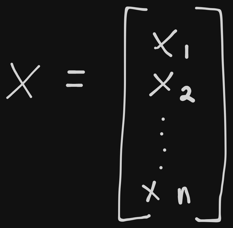
Each number is a point in space giving a coordinate point. The fact that we write it vertically instead of horizontally is purposeful, and we’ll see why later.

To slice or grab only certain elements, we can write a few different methods of notation. If we define the set $S={1, 3, 6}$, we can say that $x_s$ to refer to the elements $x_1, x_3,$ and $x_6$. We could also say $x_{-1}$ to refer to the set of all elements except for $x_1$. Similarly, $x_{-S}$ will refer to all of $x$ without the elements defined in set $S$.

Matrices

Where vectors are one dimensional arrays, matrices are two dimensional arrays. Similar rules apply for notation, this time instead of a lowercase we’ll use uppercase bold for matrices. To notate a real-valued matrix with a height or $m$ and width of $n$, we can write that as $A \in R^{m*n}$.

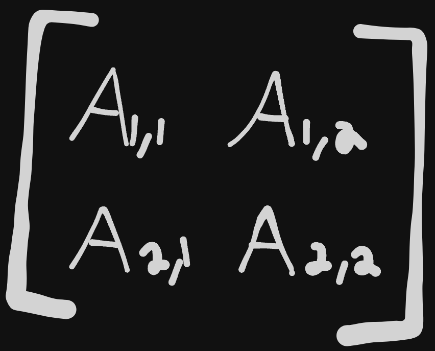
• $A_{1,1}$ returns the top left number, while $A_{m, n}$ returns the bottom right.
• : dictates horizontal coordinates; $A_{i,:}$ is the horizontal cross section of $A$, or the $i$-th row of $A$, where $A_{:,i}$ is the vertical $i$-th column of $A$.

This is a basic example of what a matrix looks like:

Tensors

Basically, a multidimensional array with more than 2 dimensions. It also uses a different typeface for identification, so for this note and all ongoing notes I’ll be using just bold with not LaTeX wrapping. We would call a tensor A, and the element of A at coordinates $(i,j,k)$ appears at A$_{i,j,k}$.

Transposing

Transposing is an operation that is common and can be done across all 4 constructs we just saw. Technically, transposing is done on matrices, so we’ll have to justify how it works for each.

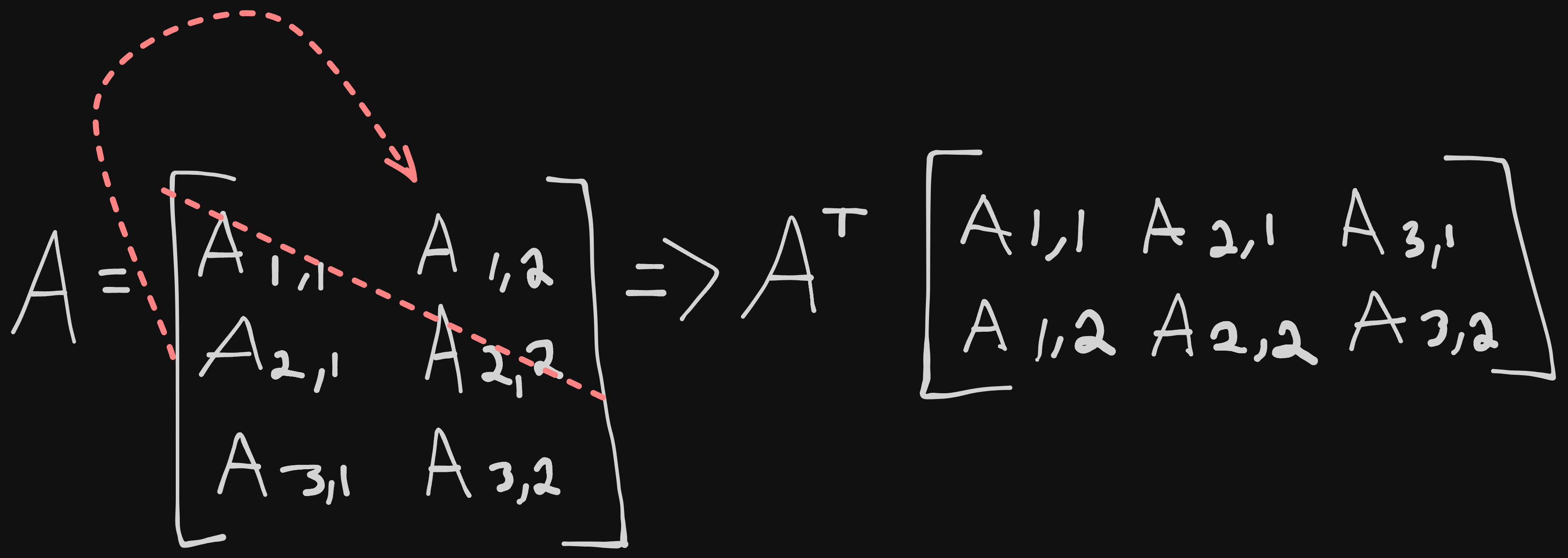
Transpose is a mirror image of a matrix dictated by the main diagonal, which is a diagonal line that runs from left to right going downwards. We denote a transposed matrix with a capital T as superscript (or \intercal in LaTeX. It sounds harder than it looks;

• Scalars are thought of a matrix with a single entry, so the transpose of a scalar is itself; $a = a^\intercal$
• Vectors are a matrix with a single column, so the transpose of a vector is a matrix with a single row. This is why writing the vector $x$ as $x=[x_1,x_2,…x_n]$ technically isn’t correct, and is actually the transposed version of $x$. For the sake of writing and not having many easy ways to horizontally, you’ll find some people write their vectors out transposed; $x=[x_1,x_2,x_3]^\intercal$.

Some very basic mathematics can be done between structures;

• Matrices can be added if they have the same shape by adding element by element; $C=A+B$ where $C_{i,j}=A_{i,j}+B_{i,j}$.
• You can add a scalar to a matrix or multiply a matrix by a scalar by moving the scalar through the matrix;
  • $D=aB+c$ where $D_{i,j}=aB+c$
• In deep learning, we can unconventionally perform the addition of a matrix and a vector, returning a separate matrix. This is done by adding the vector to each row of the matrix, otherwise known as broadcasting
  • $C=A+b$ where $C_{i,j}=A_{i,j}+b_j$

Multiplying Matrices and Vectors

There are three main types of multiplication, or products we can derive from multiplication amongst matrices; matrix product, Hadamard product, and dot product.

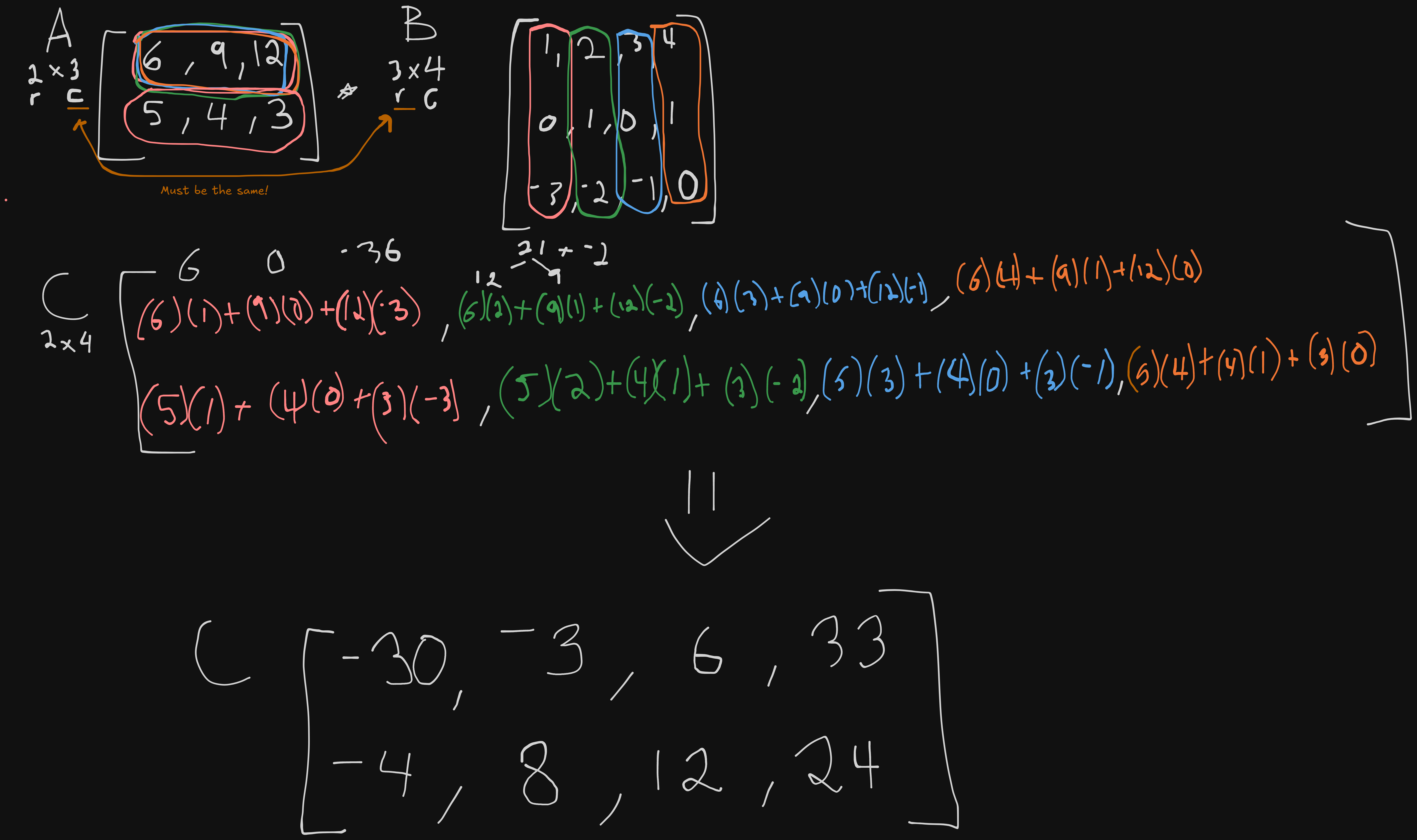
Matrix product is taking two matrices and multiplying them to create a new, third matrix. Matrix $A$ must have the same amount of columns as matrix $B$ has rows; $A$ has a shape of $mn$ while $B$ has the shape of $np$, the shape of our new matrix $C$ has a shape of $m*p$. We could also simply write this as $C=AB$.

What we’re actually doing when performing matrix multiplication is getting the dot product of our first matrices row and adding it to the product of our second matrices column and moving up from there. The actual mathematical syntax is as follows: $C_{i,j}=\sum_k A_{i,k}B_{k,j}$.

Dot product is what you think matrix multiplication is; the product of each element of a matrix against another and added together. Usually represented as $A\cdot B$.

I’ve never done matrix multiplication before, or not enough to actively remember it. Below are some examples;

Example on matrices of the same shape:

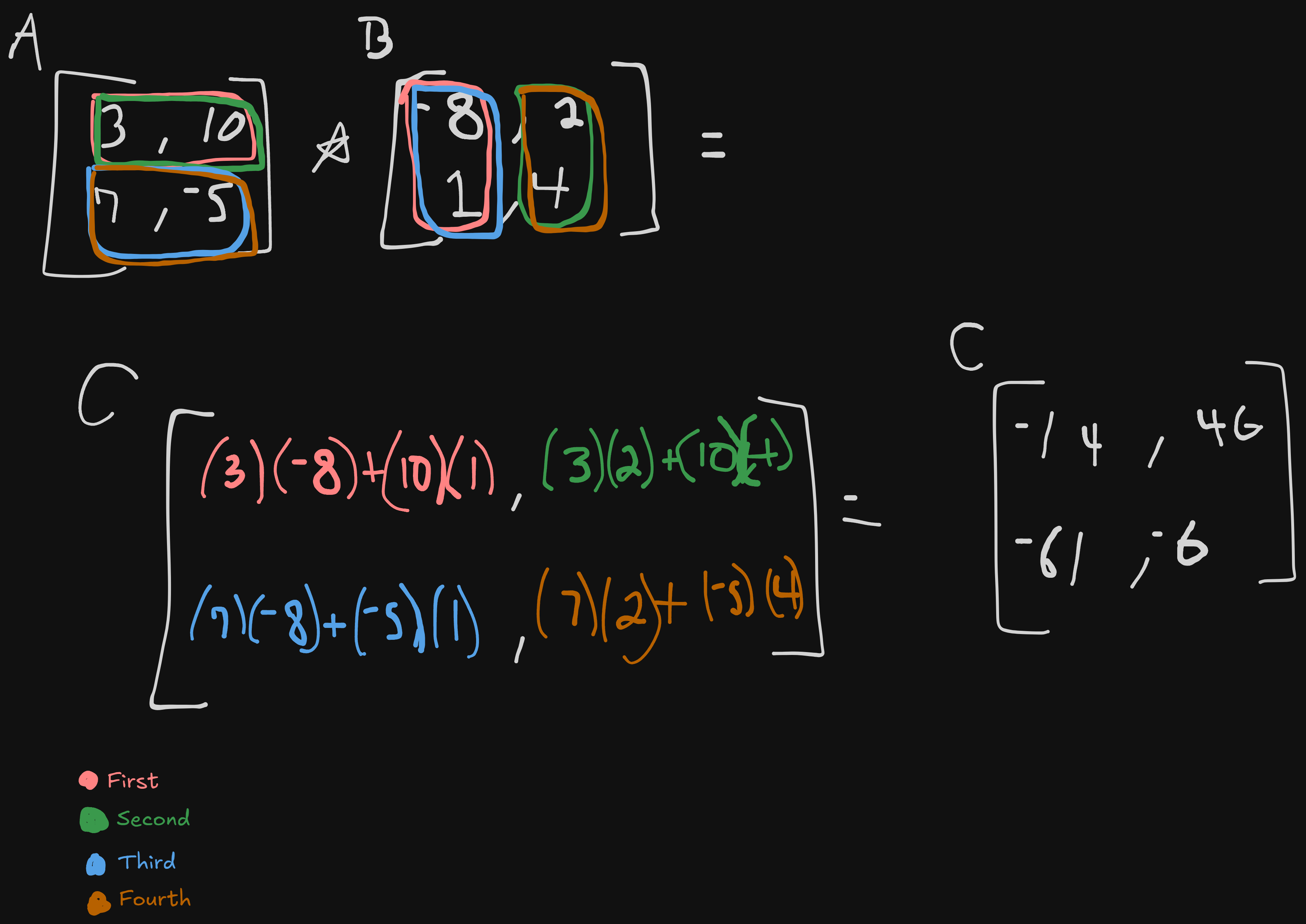
Example on matrices of different shape:

The difference between dot product and element-wise product is that in dot product, you are multiplying the components and add the products up, while in element-wise you multiply corresponding components, but don’t have to worry about summation of anything. You simply return a new vector with the same dimensions as your original vectors.

Matrix properties follow some of the properties of numbers learned in Algebra, but not all;

• Distributive
  • $A(B+C)=AB + AC$
• Associative
  • $A(BC)=(AB)C$
• NOT Commutative
  • $AB$ != $BA$
  • Dot Products between two vectors IS
    • $x\intercal y = y \intercal x$

There are more properties, but they’re not super useful at the moment so we don’t need to address them right away.

One example the text uses but doesn’t really go too in depth on is the idea of writing down a system of linear equations: $Ax=b$, where $A \in R^{m*n}$ is a known matrix, $b \in R^m$ is a known vector, and $x \in R^n$ is an unknown vector that we are trying to solve for. They mention that each row of $A$ and each element of $b$ provide another constraint, so we can rewrite $Ax=b$ as:

• $A_{1,:}x=b_1$ … $A_{2,:}x=b_2$ … $A_{m,:}x=b_m$

or even more explicitly as:

• $A_{1,1}x_1 + A_{1, 2}x_2 + … + A_{1,n}x_n=b_1$
• $A_{2,1}x_1 + A_{2, 2}x_2 + … + A_{2,n}x_n=b_2$
• $…$
• $A_{m,1}x_1 + A_{m, 2}x_2 + … + A_{m,n}x_n=b_m$

Obviously though, writing it as $Ax=b$ is a lot easier.

Identity & Inverse Matrices

This is a tough concept, so strap in. Also, so we’re on the same page, while the previous section covered vector x vector and matrix x matrix, this section is looking at our last example, which is a matrix multiplied by a vector.

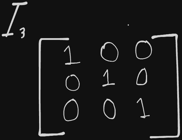
We’re going to learn about matrix inversion, which can help us understand how to solve $Ax=b$. To get there, we need to understand what an identity matrix is. An identity matrix is any matrix that when multiplied by a vector, it will not change the vector, preserving $n$-dimensional vectors as $I_n$. Therefore, $I_nx=x$. It’s quite simple to visualize; all values on the main diagonal are 1, and all other entries are 0.

Now then, the matrix inverse of $A$ would be denoted using $A^{-1}$, and actually can create an identity matrix; $A^{-1}*A=I_n$. With this, we can solve the previous system;

1. $Ax=b$
2. $A^{-1}*Ax=A^{-1}b$
3. $I_nx=A^{-1}b$
   1. We know that $I_nx=x$, so,
4. $x=A^{-1}b$

The caveat here is that all of this is only possible if we know what $A^{-1}$ is. Unfortunately, just knowing $A$ doesn’t mean we know what $A^{-1}$ is, and $A^{-1}$ might not even exist. $A^{-1}$ only exists if $A$ is a square matrix and is nonsingular (determinant is nonzero?) ((We’ll learn about this later)), therefore $A^{-1}$ is usually only useful in theory, not application.

Linear Dependence and Span

In our linear system example, in order for $A^{-1}$ to exist at all, our system must have exactly and only one solution for every value of $b$, or no/infinite solutions for $b$.

I was having trouble understanding so I threw a passage into ChatGPT to ELI5 again and it did a great job of explaining;

[! summary] Imagine you have a bunch of crayons, each a different color. Each crayon can draw a line in a different direction on a big piece of paper. Now suppose we want to draw a special point called b somewhere on the paper.

The columns of A are like different colored crayons. Each column tells you one direction you can draw a line in.

The numbers in x tell you how long (or how far) to draw with each crayon.

If you add up all these colorful lines you drew (by going exactly as far as x says in each direction), you want to land on the point b.

How many solutions the equation has is like asking: “In how many different ways can we mix these crayon lines so that the end of all our drawing lands exactly on b?

If there’s exactly one way, that means there’s only one set of crayon lengths (one set of x values) that draws a path ending on b.

If there are no ways, you can’t land on b no matter how you combine these crayons.

If there are many ways, that means you can end up on b using different sets of crayon lengths.

The above can be visualized with $Ax=\sum_i x_i A_{:,i}$, otherwise known as a linear combination. We could give it a more formal definition; any linear combination of a set of vectors {$v^{(1)},…,v^{(n)}$} can be obtained by multiplying each individual vector by a scalar coefficient and adding the results; similarly $\sum_ic_iv^{(i)}$.

Another definition to keep track of is Span, or the set of all points obtainable by linear combination of a set of vectors. Using our crayon analogy, span would be all of the points that can be made by the combination of our lines and directions.

Knowing about span let’s us understand another important aspect about $Ax=b$; to see if there is a solution, we could test is $b$ in the span of the columns making up $A$, or the range or column space of $A$.

Let’s say we have a set of vectors, and we happen to add another vector into it. If that new vector doesn’t have an outcome on the linear combination, it would be a redundant vector. This linear dependence is important; we consider a set of vectors linearly independent if each vector in the set is not a linear combination of the other vectors.

In regards to our $Ax=b$ problem, our matrix must contain at least one set of $m$ linearly independent columns. We also need to ensure we have an inverse by having at most one solution for each value of $b$, and the only way we can do so is making sure our matrix has at most $m$ columns. With both of these conditions being necessary, our matrix must be square ($m=n$) and all columns are linearly independent. Square matrix’s with linearly dependent columns are singular.

If we find that $A$ is either not a square or is singular, we can still solve it but we won’t be able to use the matrix inversion method to do so.

Norms

Norms are functions used when we need to measure the size of a given vector. We call this the $L^P$ norm, and we can formally define it as so;

$||x||{p}=(\sum{i}|x_{i}|^{p})^{1/p}$ for $p\in R, p >= 1$

What a norm is doing is mapping vectors to non-negative vectors; the norm of a vector $x$ measures the distance from the origin to the point $x$. We could get even more specific, and say that norm is any function, $f$, that abides by the following properties;

1. $f(x)=0 =>x=0$
2. $f(x+y)<=f(x)+f(y)$ (The triangle inequality)
3. $\forall \alpha \in R, f(\alpha x)=|\alpha |f(x)$

We can examine $L^2$, or $p=2$, known as the Euclidean Norm. This just measure the Euclidean distance from the origin to the point $x$. This norm is used so frequently in Machine Learning, it began being denoted as simply $||x||$, omitting the subscript of 2. Another common application is to measure the size of a given vector using the squared $L^2$ norm, calculated as $x\intercal x$.

While squared $L^2$ might be useful in some cases, in others it’s less than desirable (quite often due to how slow it increases near the origin). Another norm that is used is the $L^1$ norm, simplified as $||x||_1=\sum_i|x_i|$. We mainly use the $L^1$ norm when the difference between 0 and non 0 elements is crucial.

There also exists $L^0$, which is used when measuring the size of a vector by counting the number of non 0 elements. Some call this the $L^0$ norm, but it’s not really a norm since increasing a vector by $\alpha$ doesn’t affect the number of non 0 entries, so we use $L^1$ instead when trying to find the number of non 0 entries.

The last norm I’ll cover is $L^{\infty}$, or the max norm. This norm will simplify to the absolute value of the element with the largest magnitude in the vector; $||x||_{\infty}=max_i|x_i|$. We could also use this to find the size of a matrix, which is most commonly done with the Frobenius Norm:

$||A||F=\sqrt{\sum{i,j}A^{2}_{i,j}}$

We can also rewrite the dot product of two vectors as a norm:

$x\intercal y=||x||_2||y||_2cos\theta$ where $\theta$ = the angle between $x$ and $y$.

Special Kinds of Matrices and Vectors

Let’s go over some useful special types of matrices and vectors. The first we’ll cover is one we’ve seen slightly before- a diagonal matrix. Diagonal matrices have 0 for all entries except for the main diagonal, which contains nonzero entries. We’ve seen an example of this already with the identity matrix, which was a matrix of all 0’s except for the main diagonal of 1.

We can denote a diagonal matrix with $diag(v)$, which represents a square diagonal matrix whose diagonal entries are given by the vector $v$.

Using diagonal matrices are computationally efficient; if we wanted to compute $diag(v)x$, all we would need to do is multiply each element $x_i$ by $v_i$, which we might recognize as dot product. As long as every diagonal entry is non-zero, you can get the inverse of a diagonal matrix as well ($diag(v)^{-1}=diag([1/v_1,…,1/v_n]^{\intercal})$).

We call a matrix a Symmetric Matrix if it’s equal to it’s own transpose: $A=A^{\intercal}$.

We call any vector with a unit norm a unit vector: $||x||_2=1$.

Had to look this up, but orthogonal means “right-angled”, and we would consider two vectors, say $x$ and $y$, to be orthogonal if $x^{\intercal}y=0$. If both vectors end up having nonzero norms, they’re at a 90 degree angle to one another. In the chance that both vectors are orthogonal and also have a unit norm, we could say that they are orthonormal.

A step further, we would call any matrix a orthogonal matrix if it is square whose both rows and columns are mutually orthonormal. We could say that $A^{\intercal}A=AA^{\intercal}=I$, which implies simply that $A^{-1}=A^{\intercal}$. These are used often due to how cheap the inverse is to compute.

Eigendecomposition

Much like we can break down any number into the factors of the number to learn more about it, we can do the same for matrices. Take 12 for example. There are many ways to represent the number, but an undeniable truth regardless of the representation of the number is that $12=223$. We also learned that since this is true, every multiple of 12 will also be a multiple of 2 or 3.

We say that we decompose a matrix to find computational information about it; one of the more popular kinds of decomposition we’ll talk about is eigendecomposition, where we break down a matrix into eigenvectors and eigenvalues.

First up, an eigenvector of a square matrix, let’s say $A$, is a nonzero vector $v$ such that multiplication by $A$ will only alter the scale of $v$: $Av=\lambda v$. We use Lambda ($\lambda$) to represent the eigenvalue corresponding to said eigenvector.

If we have $v$, an eigenvector of $A$, then so too is any vector $s$, as long as $s$ is a real number and not 0. $sv$ also has the same eigenvalue, which is why we will mostly be concerned with eigenvectors.

Let’s again look at matrix $A$, suppose we have $n$ linearly independent eigenvectors {$v^{(1)},…,v^{(n)}$} along with corresponding eigenvalues {$\lambda _1,…,\lambda _n$}. We’re allowed to put all the eigenvectors together into one matrix $V$ with a single eigenvector per column: $V=[ v^{(1)},…,v^{(n)}]$. We could also put together all of the eigenvalues to form a vector $\lambda = [\lambda _1,…,\lambda _n]^{\intercal}$.

Using the above paragraph’s conclusions, we could say that the eigendecomposition of $A$ must be $A=Vdiag(\lambda)V^{-1}$.

Every real symmetric matrix can be decomposed into the following expression: $A=Q\Lambda Q^{\intercal}$, where $Q$ is an orthogonal matrix composed of eigenvectors of $A$, and $\Lambda$ is a diagonal matrix.

Some things we can learn about a matrix using eigendecomposition:

• A matrix is singular if any eigenvalues are zero
• A matrix whose eigenvalues are all positive is called a positive definite
• All positive or zero? positive semidefinite
• All negative? negative definite
• All negative or zero? negative semidefinite

Singular Value Decomposition

SVD, or singular value decomposition, is another method of factorizing a matrix, into what we call singular vectors and singular values. It will give similar information to what eigendecomposition will return, but it’s more applicable in a general sense. Any real matrix has an SVD, whereas some may not have an eigendecomposition (see non-square matrices).

In SVD, we can break down our example of matrix $A$ as $A=UDV^{\intercal}$. Again, assume $A$ is a $mn$ matrix, but this time assume $U$ as a $mm$ matrix, $D$ as a $mn$ matrix, and $V$ as an $nn$ matrix.

Not only are the sizes predetermined by the size of $A$, but each matrix also has a set structure; $U$ and $V$ are orthogonal matrices, and $D$ is a diagonal matrix. The values in the diagonal of $D$ are the singular values we were referring to earlier, while the columns of $U$ are left-singular vectors, leaving the columns of $V$ to be right-singular vectors.

The most useful feature when using SVD is when partially generalizing matrix inversion to non-square matrices (see next section).

The Moore-Penrose Pseudoinverse

There are some cases in which we will have non-square matrices that we want to use or manipulate in some way. Matrix inversion is unfortunately not defined for non-square matrices. This is where the Moore-Penrose pseudoinverse comes in.

We can use the pseudoinverse of $A$, $A^{+}=VD^{+}U^{\intercal}$, where $U, D,$ and $V$ are the SVD of $A$, and the pseudoinverse of $D^{+}$ of diagonal matrix $D$ (obtained by taking the reciprocal of the nonzero elements, then the transpose of that matrix) in situations, for example, where $A$ has more columns than rows, or vice versa.

The Trace Operator

When we want the sum of all the diagonal entries of a given matrix, we can use the Trace Operator; $Tr(A)=\sum_{i}A_{i,i}$.

There are a few instances where the Trace Operator can actually simplify some other formulas. For example, go back to our Frobenius norm, and we can make it; $||A||_F=\sqrt{Tr(AA^{\intercal})}$. It’s also useful to note that the Transpose of a Trace is equivalent; $Tr(A)=Tr(A^{\intercal})$.

When tracing a square matrix composed of multiple factors, it’s invariant to moving the last factor into the first position. Weird, but it looks like this; $Tr(ABC) = Tr(CAB) = Tr(BCA)$, which gets even further simplified to $Tr(\prod_{i=1}^{n}F^{(i)})=Tr(F^{(n)}\prod_{i=1}^{n-1}F^{(i)})$.

Trace is also invariant if the product result has a different shape; for $A\in R ^{mn}$ and $B\in R ^{nm}$, $Tr(AB)=Tr(BA)$.

The Determinant

Simply put, determinate of a square matrix ($det(A)$) isa function that maps matrices to real scalars. It can be thought of also as the product of all eigenvalues of a matrix.

Absolute value of determinants range from 0 to 1, where 0 indicates the space is contracted along one dimension, losing all volume. Conversely, 1 indicates the transformation preserves volume.

---

Next: Chapter 3